Free Statistics
of Irreproducible Research!
Description of Statistical Computation | |||||||||||||||||||||||||||||||||||||||||||||
|---|---|---|---|---|---|---|---|---|---|---|---|---|---|---|---|---|---|---|---|---|---|---|---|---|---|---|---|---|---|---|---|---|---|---|---|---|---|---|---|---|---|---|---|---|---|
| Author's title | |||||||||||||||||||||||||||||||||||||||||||||
| Author | *The author of this computation has been verified* | ||||||||||||||||||||||||||||||||||||||||||||
| R Software Module | rwasp_boxcoxlin.wasp | ||||||||||||||||||||||||||||||||||||||||||||
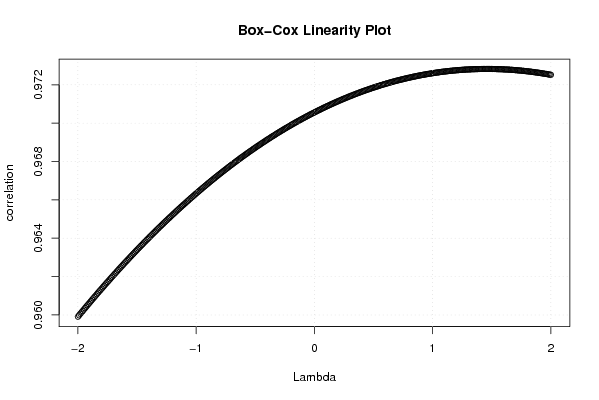
| Title produced by software | Box-Cox Linearity Plot | ||||||||||||||||||||||||||||||||||||||||||||
| Date of computation | Tue, 11 Nov 2008 14:18:29 -0700 | ||||||||||||||||||||||||||||||||||||||||||||
| Cite this page as follows | Statistical Computations at FreeStatistics.org, Office for Research Development and Education, URL https://freestatistics.org/blog/index.php?v=date/2008/Nov/11/t1226438352ky605cch3q5cpi8.htm/, Retrieved Sun, 19 May 2024 04:36:45 +0000 | ||||||||||||||||||||||||||||||||||||||||||||
| Statistical Computations at FreeStatistics.org, Office for Research Development and Education, URL https://freestatistics.org/blog/index.php?pk=23984, Retrieved Sun, 19 May 2024 04:36:45 +0000 | |||||||||||||||||||||||||||||||||||||||||||||
| QR Codes: | |||||||||||||||||||||||||||||||||||||||||||||
|
| |||||||||||||||||||||||||||||||||||||||||||||
| Original text written by user: | |||||||||||||||||||||||||||||||||||||||||||||
| IsPrivate? | No (this computation is public) | ||||||||||||||||||||||||||||||||||||||||||||
| User-defined keywords | |||||||||||||||||||||||||||||||||||||||||||||
| Estimated Impact | 147 | ||||||||||||||||||||||||||||||||||||||||||||
Tree of Dependent Computations | |||||||||||||||||||||||||||||||||||||||||||||
| Family? (F = Feedback message, R = changed R code, M = changed R Module, P = changed Parameters, D = changed Data) | |||||||||||||||||||||||||||||||||||||||||||||
| F [Univariate Data Series] [Niet werkende wer...] [2008-10-13 17:30:07] [91d2608132ba5d00ecce3524d8276757] F RMPD [Partial Correlation] [Partial Correlati...] [2008-11-11 19:49:25] [deb3c14ac9e4607a6d84fc9d0e0e6cc2] F D [Partial Correlation] [Partial Correlati...] [2008-11-11 19:56:04] [deb3c14ac9e4607a6d84fc9d0e0e6cc2] - RM D [Box-Cox Linearity Plot] [Box-Cox Linearity...] [2008-11-11 21:18:29] [5e9e099b83e50415d7642e10d74756e4] [Current] | |||||||||||||||||||||||||||||||||||||||||||||
| Feedback Forum | |||||||||||||||||||||||||||||||||||||||||||||
Post a new message | |||||||||||||||||||||||||||||||||||||||||||||
Dataset | |||||||||||||||||||||||||||||||||||||||||||||
| Dataseries X: | |||||||||||||||||||||||||||||||||||||||||||||
308347 298427 289231 291975 294912 293488 290555 284736 281818 287854 316263 325412 326011 328282 317480 317539 313737 312276 309391 302950 300316 304035 333476 337698 335932 323931 313927 314485 313218 309664 302963 298989 298423 301631 329765 335083 327616 309119 295916 291413 291542 284678 276475 272566 264981 263290 296806 303598 286994 276427 266424 267153 268381 262522 255542 253158 243803 250741 280445 285257 270976 | |||||||||||||||||||||||||||||||||||||||||||||
| Dataseries Y: | |||||||||||||||||||||||||||||||||||||||||||||
121148 114624 109822 112081 113534 112110 109826 107423 105540 108573 128591 139145 129700 132828 126868 128390 126830 124105 122323 119296 116822 119224 139357 144322 133676 128283 121640 122877 117284 116463 112685 113235 111692 113152 129889 131153 123770 112516 105940 104320 103582 99064 94989 92241 89752 90610 109456 110213 97694 91844 87572 89812 89050 85990 85070 83277 79586 84215 99708 100698 90861 | |||||||||||||||||||||||||||||||||||||||||||||
Tables (Output of Computation) | |||||||||||||||||||||||||||||||||||||||||||||
| |||||||||||||||||||||||||||||||||||||||||||||
Figures (Output of Computation) | |||||||||||||||||||||||||||||||||||||||||||||
Input Parameters & R Code | |||||||||||||||||||||||||||||||||||||||||||||
| Parameters (Session): | |||||||||||||||||||||||||||||||||||||||||||||
| Parameters (R input): | |||||||||||||||||||||||||||||||||||||||||||||
| R code (references can be found in the software module): | |||||||||||||||||||||||||||||||||||||||||||||
n <- length(x) | |||||||||||||||||||||||||||||||||||||||||||||