Free Statistics
of Irreproducible Research!
Description of Statistical Computation | |||||||||||||||||||||||||||||||||||||||||||||
|---|---|---|---|---|---|---|---|---|---|---|---|---|---|---|---|---|---|---|---|---|---|---|---|---|---|---|---|---|---|---|---|---|---|---|---|---|---|---|---|---|---|---|---|---|---|
| Author's title | |||||||||||||||||||||||||||||||||||||||||||||
| Author | *Unverified author* | ||||||||||||||||||||||||||||||||||||||||||||
| R Software Module | rwasp_boxcoxlin.wasp | ||||||||||||||||||||||||||||||||||||||||||||
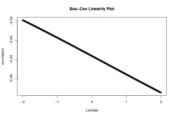
| Title produced by software | Box-Cox Linearity Plot | ||||||||||||||||||||||||||||||||||||||||||||
| Date of computation | Thu, 13 Nov 2008 14:13:17 -0700 | ||||||||||||||||||||||||||||||||||||||||||||
| Cite this page as follows | Statistical Computations at FreeStatistics.org, Office for Research Development and Education, URL https://freestatistics.org/blog/index.php?v=date/2008/Nov/13/t122661083109m6vqb32gcti0u.htm/, Retrieved Sun, 19 May 2024 04:51:59 +0000 | ||||||||||||||||||||||||||||||||||||||||||||
| Statistical Computations at FreeStatistics.org, Office for Research Development and Education, URL https://freestatistics.org/blog/index.php?pk=24835, Retrieved Sun, 19 May 2024 04:51:59 +0000 | |||||||||||||||||||||||||||||||||||||||||||||
| QR Codes: | |||||||||||||||||||||||||||||||||||||||||||||
|
| |||||||||||||||||||||||||||||||||||||||||||||
| Original text written by user: | |||||||||||||||||||||||||||||||||||||||||||||
| IsPrivate? | No (this computation is public) | ||||||||||||||||||||||||||||||||||||||||||||
| User-defined keywords | kleuter | ||||||||||||||||||||||||||||||||||||||||||||
| Estimated Impact | 163 | ||||||||||||||||||||||||||||||||||||||||||||
Tree of Dependent Computations | |||||||||||||||||||||||||||||||||||||||||||||
| Family? (F = Feedback message, R = changed R code, M = changed R Module, P = changed Parameters, D = changed Data) | |||||||||||||||||||||||||||||||||||||||||||||
| - [Box-Cox Linearity Plot] [] [2008-11-13 21:13:17] [b5c0979bf79a38ace87e0d3abace1ca1] [Current] | |||||||||||||||||||||||||||||||||||||||||||||
| Feedback Forum | |||||||||||||||||||||||||||||||||||||||||||||
Post a new message | |||||||||||||||||||||||||||||||||||||||||||||
Dataset | |||||||||||||||||||||||||||||||||||||||||||||
| Dataseries X: | |||||||||||||||||||||||||||||||||||||||||||||
9,4 9,5 9,1 9 9,3 9,9 9,8 9,4 8,3 8 8,5 10,4 11,1 10,9 9,9 9,2 9,2 9,5 9,6 9,5 9,1 8,9 9 10,1 10,3 10,2 9,6 9,2 9,3 9,4 9,4 9,2 9 9 9 9,8 10 9,9 9,3 9 9 9,1 9,1 9,1 9,2 8,8 8,3 8,4 8,1 7,8 7,9 7,9 8 7,9 7,5 7,2 6,9 6,6 6,7 7,3 7,5 | |||||||||||||||||||||||||||||||||||||||||||||
| Dataseries Y: | |||||||||||||||||||||||||||||||||||||||||||||
63,3 102,9 107,6 93 84,1 89,7 90,1 103,4 95,6 90,4 104,1 82,8 69 105,1 104,3 95,4 93 89,3 85,2 96,4 93,1 83,3 98,4 76,9 66,3 98,6 92,3 96,1 84,4 85,8 94,6 101,5 86 91,1 101,8 79,4 67,3 98,1 104,7 102,9 82,8 94,5 93,1 103,6 89,9 92,5 103,5 86,9 69,5 97,1 109,8 96,6 75,8 127,5 93,4 87,7 94 84 90,1 81,5 58,6 | |||||||||||||||||||||||||||||||||||||||||||||
Tables (Output of Computation) | |||||||||||||||||||||||||||||||||||||||||||||
| |||||||||||||||||||||||||||||||||||||||||||||
Figures (Output of Computation) | |||||||||||||||||||||||||||||||||||||||||||||
Input Parameters & R Code | |||||||||||||||||||||||||||||||||||||||||||||
| Parameters (Session): | |||||||||||||||||||||||||||||||||||||||||||||
| Parameters (R input): | |||||||||||||||||||||||||||||||||||||||||||||
| R code (references can be found in the software module): | |||||||||||||||||||||||||||||||||||||||||||||
n <- length(x) | |||||||||||||||||||||||||||||||||||||||||||||