Free Statistics

of Irreproducible Research!

Author's title

Author*The author of this computation has been verified*
R Software Modulerwasp_boxcoxnorm.wasp
Title produced by softwareBox-Cox Normality Plot
Date of computationMon, 27 Oct 2008 11:17:39 -0600
Cite this page as followsStatistical Computations at FreeStatistics.org, Office for Research Development and Education, URL https://freestatistics.org/blog/index.php?v=date/2008/Oct/27/t1225127963dkqnd9p5bo0sw5f.htm/, Retrieved Sun, 26 May 2024 09:38:41 +0000
Statistical Computations at FreeStatistics.org, Office for Research Development and Education, URL https://freestatistics.org/blog/index.php?pk=19284, Retrieved Sun, 26 May 2024 09:38:41 +0000
QR Codes:

Original text written by user:
IsPrivate?No (this computation is public)
User-defined keywordsBox-Cox plot vervaardigde kleding
Estimated Impact128
Family? (F = Feedback message, R = changed R code, M = changed R Module, P = changed Parameters, D = changed Data)
-       [Box-Cox Normality Plot] [Box-Cox plot verv...] [2008-10-27 17:17:39] [f4b2017b314c03698059f43b95818e67] [Current]
Feedback Forum

Post a new message
Dataseries X:
110.40
96.40
101.90
106.20
81.00
94.70
101.00
109.40
102.30
90.70
96.20
96.10
106.00
103.10
102.00
104.70
86.00
92.10
106.90
112.60
101.70
92.00
97.40
97.00
105.40
102.70
98.10
104.50
87.40
89.90
109.80
111.70
98.60
96.90
95.10
97.00
112.70
102.90
97.40
111.40
87.40
96.80
114.10
110.30
103.90
101.60
94.60
95.90
104.70
102.80
98.10
113.90
80.90
95.70
113.20
105.90
108.80
102.30
99.00
100.70
115.50


Summary of computational transaction
Raw Inputview raw input (R code)
Raw Outputview raw output of R engine
Computing time4 seconds
R Server'Gwilym Jenkins' @ 72.249.127.135

\begin{tabular}{lllllllll}
\hline
Summary of computational transaction \tabularnewline
Raw Input & view raw input (R code)  \tabularnewline
Raw Output & view raw output of R engine  \tabularnewline
Computing time & 4 seconds \tabularnewline
R Server & 'Gwilym Jenkins' @ 72.249.127.135 \tabularnewline
\hline
\end{tabular}
%Source: https://freestatistics.org/blog/index.php?pk=19284&T=0

[TABLE]
[ROW][C]Summary of computational transaction[/C][/ROW]
[ROW][C]Raw Input[/C][C]view raw input (R code) [/C][/ROW]
[ROW][C]Raw Output[/C][C]view raw output of R engine [/C][/ROW]
[ROW][C]Computing time[/C][C]4 seconds[/C][/ROW]
[ROW][C]R Server[/C][C]'Gwilym Jenkins' @ 72.249.127.135[/C][/ROW]
[/TABLE]
Source: https://freestatistics.org/blog/index.php?pk=19284&T=0

Globally Unique Identifier (entire table): ba.freestatistics.org/blog/index.php?pk=19284&T=0

As an alternative you can also use a QR Code:  

The GUIDs for individual cells are displayed in the table below:

Summary of computational transaction
Raw Inputview raw input (R code)
Raw Outputview raw output of R engine
Computing time4 seconds
R Server'Gwilym Jenkins' @ 72.249.127.135


Box-Cox Normality Plot
# observations x61
maximum correlation0.170091861483865
optimal lambda2

\begin{tabular}{lllllllll}
\hline
Box-Cox Normality Plot \tabularnewline
# observations x & 61 \tabularnewline
maximum correlation & 0.170091861483865 \tabularnewline
optimal lambda & 2 \tabularnewline
\hline
\end{tabular}
%Source: https://freestatistics.org/blog/index.php?pk=19284&T=1

[TABLE]
[ROW][C]Box-Cox Normality Plot[/C][/ROW]
[ROW][C]# observations x[/C][C]61[/C][/ROW]
[ROW][C]maximum correlation[/C][C]0.170091861483865[/C][/ROW]
[ROW][C]optimal lambda[/C][C]2[/C][/ROW]
[/TABLE]
Source: https://freestatistics.org/blog/index.php?pk=19284&T=1

Globally Unique Identifier (entire table): ba.freestatistics.org/blog/index.php?pk=19284&T=1

As an alternative you can also use a QR Code:  

The GUIDs for individual cells are displayed in the table below:

Box-Cox Normality Plot
# observations x61
maximum correlation0.170091861483865
optimal lambda2


Parameters (Session):
Parameters (R input):
R code (references can be found in the software module):
n <- length(x)
c <- array(NA,dim=c(401))
l <- array(NA,dim=c(401))
mx <- 0
mxli <- -999
for (i in 1:401)
{
l[i] <- (i-201)/100
if (l[i] != 0)
{
x1 <- (x^l[i] - 1) / l[i]
} else {
x1 <- log(x)
}
c[i] <- cor(qnorm(ppoints(x), mean=0, sd=1),x1)
if (mx < c[i])
{
mx <- c[i]
mxli <- l[i]
}
}
c
mx
mxli
if (mxli != 0)
{
x1 <- (x^mxli - 1) / mxli
} else {
x1 <- log(x)
}
bitmap(file='test1.png')
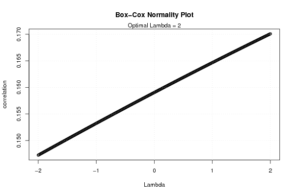
plot(l,c,main='Box-Cox Normality Plot',xlab='Lambda',ylab='correlation')
mtext(paste('Optimal Lambda =',mxli))
grid()
dev.off()
bitmap(file='test2.png')
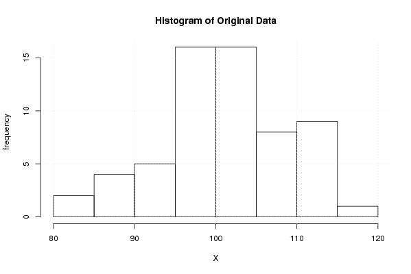
hist(x,main='Histogram of Original Data',xlab='X',ylab='frequency')
grid()
dev.off()
bitmap(file='test3.png')
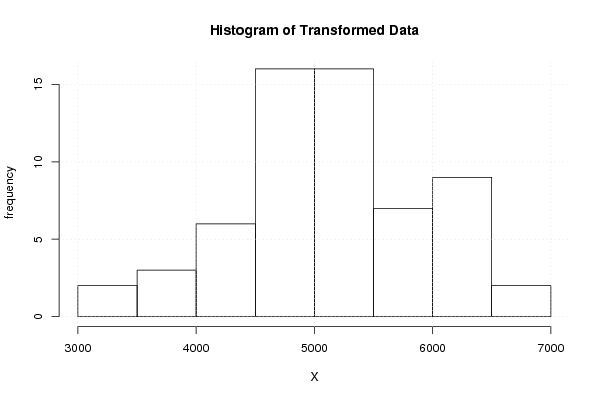
hist(x1,main='Histogram of Transformed Data',xlab='X',ylab='frequency')
grid()
dev.off()
bitmap(file='test4.png')
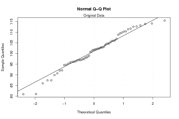
qqnorm(x)
qqline(x)
grid()
mtext('Original Data')
dev.off()
bitmap(file='test5.png')
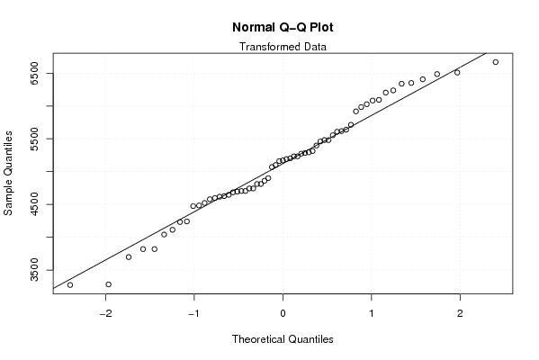
qqnorm(x1)
qqline(x1)
grid()
mtext('Transformed Data')
dev.off()
load(file='createtable')
a<-table.start()
a<-table.row.start(a)
a<-table.element(a,'Box-Cox Normality Plot',2,TRUE)
a<-table.row.end(a)
a<-table.row.start(a)
a<-table.element(a,'# observations x',header=TRUE)
a<-table.element(a,n)
a<-table.row.end(a)
a<-table.row.start(a)
a<-table.element(a,'maximum correlation',header=TRUE)
a<-table.element(a,mx)
a<-table.row.end(a)
a<-table.row.start(a)
a<-table.element(a,'optimal lambda',header=TRUE)
a<-table.element(a,mxli)
a<-table.row.end(a)
a<-table.end(a)
table.save(a,file='mytable.tab')