Free Statistics
of Irreproducible Research!
Description of Statistical Computation | |||||||||||||||||||||||||||||||||||||||||||||||||||||
|---|---|---|---|---|---|---|---|---|---|---|---|---|---|---|---|---|---|---|---|---|---|---|---|---|---|---|---|---|---|---|---|---|---|---|---|---|---|---|---|---|---|---|---|---|---|---|---|---|---|---|---|---|---|
| Author's title | |||||||||||||||||||||||||||||||||||||||||||||||||||||
| Author | *The author of this computation has been verified* | ||||||||||||||||||||||||||||||||||||||||||||||||||||
| R Software Module | rwasp_edauni.wasp | ||||||||||||||||||||||||||||||||||||||||||||||||||||
| Title produced by software | Univariate Explorative Data Analysis | ||||||||||||||||||||||||||||||||||||||||||||||||||||
| Date of computation | Mon, 27 Oct 2008 15:31:04 -0600 | ||||||||||||||||||||||||||||||||||||||||||||||||||||
| Cite this page as follows | Statistical Computations at FreeStatistics.org, Office for Research Development and Education, URL https://freestatistics.org/blog/index.php?v=date/2008/Oct/27/t1225143217nwiwx7npjtty2vy.htm/, Retrieved Sun, 19 May 2024 00:26:35 +0000 | ||||||||||||||||||||||||||||||||||||||||||||||||||||
| Statistical Computations at FreeStatistics.org, Office for Research Development and Education, URL https://freestatistics.org/blog/index.php?pk=19642, Retrieved Sun, 19 May 2024 00:26:35 +0000 | |||||||||||||||||||||||||||||||||||||||||||||||||||||
| QR Codes: | |||||||||||||||||||||||||||||||||||||||||||||||||||||
|
| |||||||||||||||||||||||||||||||||||||||||||||||||||||
| Original text written by user: | |||||||||||||||||||||||||||||||||||||||||||||||||||||
| IsPrivate? | No (this computation is public) | ||||||||||||||||||||||||||||||||||||||||||||||||||||
| User-defined keywords | |||||||||||||||||||||||||||||||||||||||||||||||||||||
| Estimated Impact | 141 | ||||||||||||||||||||||||||||||||||||||||||||||||||||
Tree of Dependent Computations | |||||||||||||||||||||||||||||||||||||||||||||||||||||
| Family? (F = Feedback message, R = changed R code, M = changed R Module, P = changed Parameters, D = changed Data) | |||||||||||||||||||||||||||||||||||||||||||||||||||||
| F [Univariate Explorative Data Analysis] [Q7] [2008-10-27 21:31:04] [5e2b1e7aa808f9f0d23fd35605d4968f] [Current] - P [Univariate Explorative Data Analysis] [Q7 correctie] [2008-11-01 18:11:19] [547636b63517c1c2916a747d66b36ebf] - P [Univariate Explorative Data Analysis] [Q7 - verbetering] [2008-11-02 14:54:25] [299afd6311e4c20059ea2f05c8dd029d] - RM [Harrell-Davis Quantiles] [Q9] [2008-11-02 15:18:12] [299afd6311e4c20059ea2f05c8dd029d] - R [Harrell-Davis Quantiles] [Q9 - wijziging R-...] [2008-11-02 15:27:37] [299afd6311e4c20059ea2f05c8dd029d] | |||||||||||||||||||||||||||||||||||||||||||||||||||||
| Feedback Forum | |||||||||||||||||||||||||||||||||||||||||||||||||||||
Post a new message | |||||||||||||||||||||||||||||||||||||||||||||||||||||
Dataset | |||||||||||||||||||||||||||||||||||||||||||||||||||||
| Dataseries X: | |||||||||||||||||||||||||||||||||||||||||||||||||||||
12192.5 11268.8 9097.4 12639.8 13040.1 11687.3 11191.7 11391.9 11793.1 13933.2 12778.1 11810.3 13698.4 11956.6 10723.8 13938.9 13979.8 13807.4 12973.9 12509.8 12934.1 14908.3 13772.1 13012.6 14049.9 11816.5 11593.2 14466.2 13615.9 14733.9 13880.7 13527.5 13584.0 16170.2 13260.6 14741.9 15486.5 13154.5 12621.2 15031.6 15452.4 15428.0 13105.9 14716.8 14180.0 16202.2 14392.4 15140.6 15960.1 14351.3 13230.2 15202.1 17157.3 16159.1 13405.7 17224.7 17338.4 17370.6 18817.8 16593.2 17979.5 | |||||||||||||||||||||||||||||||||||||||||||||||||||||
Tables (Output of Computation) | |||||||||||||||||||||||||||||||||||||||||||||||||||||
| |||||||||||||||||||||||||||||||||||||||||||||||||||||
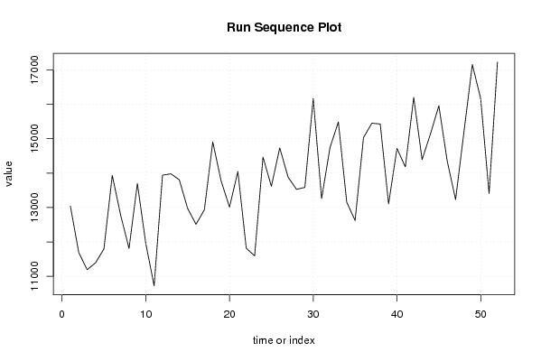
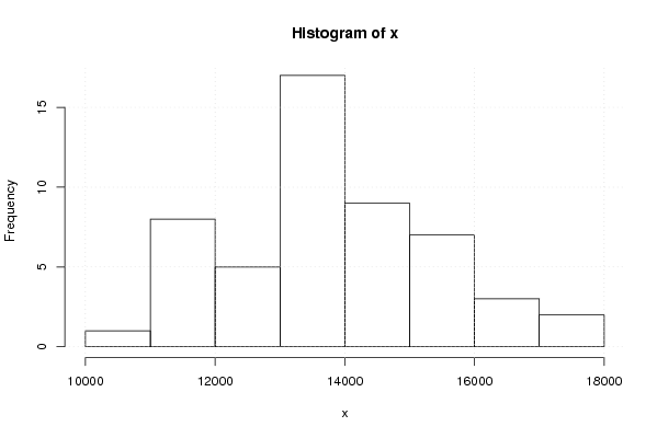
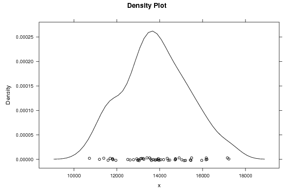
Figures (Output of Computation) | |||||||||||||||||||||||||||||||||||||||||||||||||||||
Input Parameters & R Code | |||||||||||||||||||||||||||||||||||||||||||||||||||||
| Parameters (Session): | |||||||||||||||||||||||||||||||||||||||||||||||||||||
| par1 = 0 ; par2 = 0 ; | |||||||||||||||||||||||||||||||||||||||||||||||||||||
| Parameters (R input): | |||||||||||||||||||||||||||||||||||||||||||||||||||||
| par1 = 0 ; par2 = 0 ; | |||||||||||||||||||||||||||||||||||||||||||||||||||||
| R code (references can be found in the software module): | |||||||||||||||||||||||||||||||||||||||||||||||||||||
par1 <- as.numeric(par1) | |||||||||||||||||||||||||||||||||||||||||||||||||||||