Free Statistics
of Irreproducible Research!
Description of Statistical Computation | |||||||||||||||||||||
|---|---|---|---|---|---|---|---|---|---|---|---|---|---|---|---|---|---|---|---|---|---|
| Author's title | |||||||||||||||||||||
| Author | *The author of this computation has been verified* | ||||||||||||||||||||
| R Software Module | rwasp_meanplot.wasp | ||||||||||||||||||||
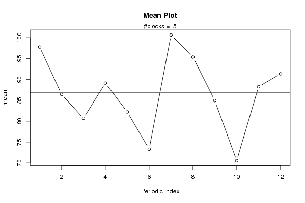
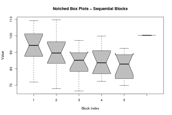
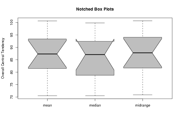
| Title produced by software | Mean Plot | ||||||||||||||||||||
| Date of computation | Thu, 30 Oct 2008 06:55:29 -0600 | ||||||||||||||||||||
| Cite this page as follows | Statistical Computations at FreeStatistics.org, Office for Research Development and Education, URL https://freestatistics.org/blog/index.php?v=date/2008/Oct/30/t12253713654d6604ffzlnpj67.htm/, Retrieved Sat, 18 May 2024 10:35:20 +0000 | ||||||||||||||||||||
| Statistical Computations at FreeStatistics.org, Office for Research Development and Education, URL https://freestatistics.org/blog/index.php?pk=19999, Retrieved Sat, 18 May 2024 10:35:20 +0000 | |||||||||||||||||||||
| QR Codes: | |||||||||||||||||||||
|
| |||||||||||||||||||||
| Original text written by user: | |||||||||||||||||||||
| IsPrivate? | No (this computation is public) | ||||||||||||||||||||
| User-defined keywords | |||||||||||||||||||||
| Estimated Impact | 217 | ||||||||||||||||||||
Tree of Dependent Computations | |||||||||||||||||||||
| Family? (F = Feedback message, R = changed R code, M = changed R Module, P = changed Parameters, D = changed Data) | |||||||||||||||||||||
| F [Mean Plot] [workshop 3] [2007-10-26 12:14:28] [e9ffc5de6f8a7be62f22b142b5b6b1a8] F D [Mean Plot] [taak 4 - Q2 Boxplot] [2008-10-30 12:55:29] [b23db733701c4d62df5e228d507c1c6a] [Current] F R [Mean Plot] [taak 4 - task 4(1)] [2008-10-30 14:19:16] [46c5a5fbda57fdfa1d4ef48658f82a0c] - [Mean Plot] [Task 4, Result 1] [2008-10-31 12:39:54] [70cb582895831af4be81fec73c607e93] - [Mean Plot] [TAAK 4] [2008-10-31 12:49:51] [29647dffafb5b58c12a48dbf6cba2b57] - D [Mean Plot] [taak 4 - task 5] [2008-10-30 14:36:35] [46c5a5fbda57fdfa1d4ef48658f82a0c] - D [Mean Plot] [Task 5, Result 2] [2008-10-31 12:49:54] [70cb582895831af4be81fec73c607e93] - D [Mean Plot] [Task 2, Result 3] [2008-10-31 13:00:11] [70cb582895831af4be81fec73c607e93] F D [Mean Plot] [Taak 5-2] [2008-10-31 13:12:40] [29647dffafb5b58c12a48dbf6cba2b57] - RM D [Star Plot] [taak 4 part 2 Q2 ...] [2008-10-30 15:05:10] [46c5a5fbda57fdfa1d4ef48658f82a0c] - P [Star Plot] [star plot part 2 q2] [2008-10-30 15:24:47] [e620d6a6dfa1ac8b8fa0baf96d77e822] F P [Star Plot] [part 2 q2] [2008-10-30 15:24:47] [e1a46c1dcfccb0cb690f79a1a409b517] - RMPD [Mean Plot] [part 2 q3] [2008-10-30 15:49:15] [e1a46c1dcfccb0cb690f79a1a409b517] F D [Mean Plot] [part 2 q3 ] [2008-10-30 16:03:45] [e1a46c1dcfccb0cb690f79a1a409b517] - D [Mean Plot] [part 2 q3] [2008-10-30 16:06:27] [e1a46c1dcfccb0cb690f79a1a409b517] - D [Mean Plot] [part 2 q3] [2008-10-30 16:09:00] [e1a46c1dcfccb0cb690f79a1a409b517] - D [Mean Plot] [part 2 q3] [2008-10-30 16:12:00] [e1a46c1dcfccb0cb690f79a1a409b517] - [Star Plot] [Part 2, Task 1, Q1] [2008-10-31 13:25:18] [70cb582895831af4be81fec73c607e93] - P [Star Plot] [Q2 Hypothesis Tes...] [2008-10-31 13:56:43] [29647dffafb5b58c12a48dbf6cba2b57] - PD [Star Plot] [Star Plot: Auto's] [2008-11-03 09:24:24] [b5373f20234c18c6452d5f98d8abf0fe] - R D [Mean Plot] [taak 4 part 2 Q3 ...] [2008-10-30 15:43:11] [46c5a5fbda57fdfa1d4ef48658f82a0c] - D [Mean Plot] [Deel 2, Task 1, Q3] [2008-10-31 13:27:50] [70cb582895831af4be81fec73c607e93] F D [Mean Plot] [Q3 Hypothesis Tes...] [2008-10-31 14:51:36] [29647dffafb5b58c12a48dbf6cba2b57] - R D [Mean Plot] [taak 4 part 2 Q3 ...] [2008-10-30 15:45:34] [46c5a5fbda57fdfa1d4ef48658f82a0c] - D [Mean Plot] [taak 4 part 2 Q3 ...] [2008-10-30 15:47:17] [46c5a5fbda57fdfa1d4ef48658f82a0c] - D [Mean Plot] [Deel 2, Task 1, Q3] [2008-10-31 13:34:36] [70cb582895831af4be81fec73c607e93] F D [Mean Plot] [Q3 Hypothesis Tes...] [2008-10-31 14:56:26] [29647dffafb5b58c12a48dbf6cba2b57] - D [Mean Plot] [taak 4 part 2 Q3 ...] [2008-10-30 15:48:28] [46c5a5fbda57fdfa1d4ef48658f82a0c] - D [Mean Plot] [Deel 2, Task 1, Q3] [2008-10-31 13:36:14] [70cb582895831af4be81fec73c607e93] F D [Mean Plot] [Q3 Hypothesis Tes...] [2008-10-31 14:58:33] [29647dffafb5b58c12a48dbf6cba2b57] - D [Mean Plot] [taak 4 part 2 Q3 ...] [2008-10-30 15:49:57] [46c5a5fbda57fdfa1d4ef48658f82a0c] - D [Mean Plot] [Deel 2, Task 1, Q3] [2008-10-31 13:37:59] [70cb582895831af4be81fec73c607e93] F D [Mean Plot] [Q3 Hypothesis Tes...] [2008-10-31 15:00:35] [29647dffafb5b58c12a48dbf6cba2b57] - D [Mean Plot] [Deel 2, Task 1, Q3] [2008-10-31 13:29:09] [70cb582895831af4be81fec73c607e93] F D [Mean Plot] [Q3 Hypothesis Tes...] [2008-10-31 14:54:00] [29647dffafb5b58c12a48dbf6cba2b57] - [Mean Plot] [Task 1, result 2] [2008-10-31 12:24:56] [70cb582895831af4be81fec73c607e93] F [Mean Plot] [TAAK 1 Q2] [2008-10-31 12:28:40] [29647dffafb5b58c12a48dbf6cba2b57] F R [Mean Plot] [Mean Plot] [2008-11-03 08:20:36] [b5373f20234c18c6452d5f98d8abf0fe] - [Mean Plot] [Task 1, Result 3] [2008-10-31 12:27:38] [70cb582895831af4be81fec73c607e93] F [Mean Plot] [TAAK 1 Q3] [2008-10-31 12:32:30] [29647dffafb5b58c12a48dbf6cba2b57] F R D [Mean Plot] [Mean Plot Q3] [2008-11-03 08:28:27] [b5373f20234c18c6452d5f98d8abf0fe] - D [Mean Plot] [Algemeen Economis...] [2008-12-13 12:10:56] [70cb582895831af4be81fec73c607e93] - D [Mean Plot] [Financi�le situat...] [2008-12-13 12:31:20] [70cb582895831af4be81fec73c607e93] - D [Mean Plot] [Indicator consume...] [2008-12-13 12:43:15] [70cb582895831af4be81fec73c607e93] - D [Mean Plot] [Notched Box Plots...] [2008-12-15 23:20:10] [70cb582895831af4be81fec73c607e93] | |||||||||||||||||||||
| Feedback Forum | |||||||||||||||||||||
Post a new message | |||||||||||||||||||||
Dataset | |||||||||||||||||||||
| Dataseries X: | |||||||||||||||||||||
109.20 88.60 94.30 98.30 86.40 80.60 104.10 108.20 93.40 71.90 94.10 94.90 96.40 91.10 84.40 86.40 88.00 75.10 109.70 103.00 82.10 68.00 96.40 94.30 90.00 88.00 76.10 82.50 81.40 66.50 97.20 94.10 80.70 70.50 87.80 89.50 99.60 84.20 75.10 92.00 80.80 73.10 99.80 90.00 83.10 72.40 78.80 87.30 91.00 80.10 73.60 86.40 74.50 71.20 92.40 81.50 85.30 69.90 84.20 90.70 100.30 | |||||||||||||||||||||
Tables (Output of Computation) | |||||||||||||||||||||
| |||||||||||||||||||||
Figures (Output of Computation) | |||||||||||||||||||||
Input Parameters & R Code | |||||||||||||||||||||
| Parameters (Session): | |||||||||||||||||||||
| par1 = 12 ; | |||||||||||||||||||||
| Parameters (R input): | |||||||||||||||||||||
| par1 = 12 ; | |||||||||||||||||||||
| R code (references can be found in the software module): | |||||||||||||||||||||
par1 <- as.numeric(par1) | |||||||||||||||||||||