Free Statistics
of Irreproducible Research!
Description of Statistical Computation | |||||||||||||||||||||||||||||||||||||||||||||||||||||
|---|---|---|---|---|---|---|---|---|---|---|---|---|---|---|---|---|---|---|---|---|---|---|---|---|---|---|---|---|---|---|---|---|---|---|---|---|---|---|---|---|---|---|---|---|---|---|---|---|---|---|---|---|---|
| Author's title | |||||||||||||||||||||||||||||||||||||||||||||||||||||
| Author | *The author of this computation has been verified* | ||||||||||||||||||||||||||||||||||||||||||||||||||||
| R Software Module | rwasp_edauni.wasp | ||||||||||||||||||||||||||||||||||||||||||||||||||||
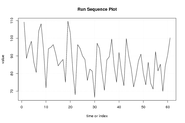
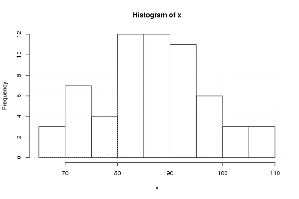
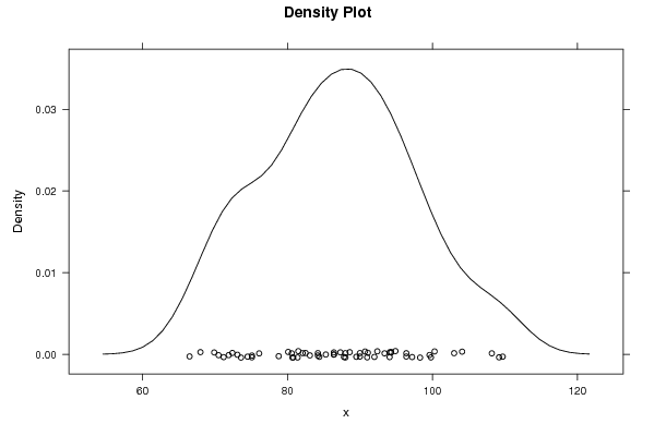
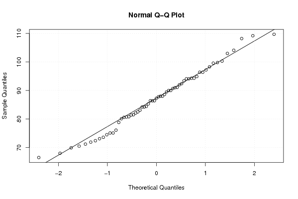
| Title produced by software | Univariate Explorative Data Analysis | ||||||||||||||||||||||||||||||||||||||||||||||||||||
| Date of computation | Fri, 31 Oct 2008 13:26:40 -0600 | ||||||||||||||||||||||||||||||||||||||||||||||||||||
| Cite this page as follows | Statistical Computations at FreeStatistics.org, Office for Research Development and Education, URL https://freestatistics.org/blog/index.php?v=date/2008/Oct/31/t1225481296kec92gedvc53vqz.htm/, Retrieved Sat, 18 May 2024 16:27:40 +0000 | ||||||||||||||||||||||||||||||||||||||||||||||||||||
| Statistical Computations at FreeStatistics.org, Office for Research Development and Education, URL https://freestatistics.org/blog/index.php?pk=20314, Retrieved Sat, 18 May 2024 16:27:40 +0000 | |||||||||||||||||||||||||||||||||||||||||||||||||||||
| QR Codes: | |||||||||||||||||||||||||||||||||||||||||||||||||||||
|
| |||||||||||||||||||||||||||||||||||||||||||||||||||||
| Original text written by user: | |||||||||||||||||||||||||||||||||||||||||||||||||||||
| IsPrivate? | No (this computation is public) | ||||||||||||||||||||||||||||||||||||||||||||||||||||
| User-defined keywords | |||||||||||||||||||||||||||||||||||||||||||||||||||||
| Estimated Impact | 210 | ||||||||||||||||||||||||||||||||||||||||||||||||||||
Tree of Dependent Computations | |||||||||||||||||||||||||||||||||||||||||||||||||||||
| Family? (F = Feedback message, R = changed R code, M = changed R Module, P = changed Parameters, D = changed Data) | |||||||||||||||||||||||||||||||||||||||||||||||||||||
| F [Univariate Explorative Data Analysis] [Q2 IA2] [2008-10-27 18:55:20] [3d2d096cc21c6f80db3dd7b8e12effce] - PD [Univariate Explorative Data Analysis] [Q2 Univariate Exp...] [2008-10-31 19:26:40] [35348cd8592af0baf5f138bd59921307] [Current] - RMP [Central Tendency] [Q2 Central Tendency] [2008-11-01 09:55:04] [7d3039e6253bb5fb3b26df1537d500b4] - [Central Tendency] [verbetering Q2 IA2] [2008-11-03 15:48:49] [3d2d096cc21c6f80db3dd7b8e12effce] - P [Univariate Explorative Data Analysis] [Q2 Univariate Exp...] [2008-11-01 13:45:41] [7d3039e6253bb5fb3b26df1537d500b4] - [Univariate Explorative Data Analysis] [Q2 Univariate Exp...] [2008-11-02 11:22:14] [c993f605b206b366f754f7f8c1fcc291] - P [Univariate Explorative Data Analysis] [Q2 Univariate Exp...] [2008-11-02 11:55:51] [c993f605b206b366f754f7f8c1fcc291] | |||||||||||||||||||||||||||||||||||||||||||||||||||||
| Feedback Forum | |||||||||||||||||||||||||||||||||||||||||||||||||||||
Post a new message | |||||||||||||||||||||||||||||||||||||||||||||||||||||
Dataset | |||||||||||||||||||||||||||||||||||||||||||||||||||||
| Dataseries X: | |||||||||||||||||||||||||||||||||||||||||||||||||||||
109.20 88.60 94.30 98.30 86.40 80.60 104.10 108.20 93.40 71.90 94.10 94.90 96.40 91.10 84.40 86.40 88.00 75.10 109.70 103.00 82.10 68.00 96.40 94.30 90.00 88.00 76.10 82.50 81.40 66.50 97.20 94.10 80.70 70.50 87.80 89.50 99.60 84.20 75.10 92.00 80.80 73.10 99.80 90.00 83.10 72.40 78.80 87.30 91.00 80.10 73.60 86.40 74.50 71.20 92.40 81.50 85.30 69.90 84.20 90.70 100.30 | |||||||||||||||||||||||||||||||||||||||||||||||||||||
Tables (Output of Computation) | |||||||||||||||||||||||||||||||||||||||||||||||||||||
| |||||||||||||||||||||||||||||||||||||||||||||||||||||
Figures (Output of Computation) | |||||||||||||||||||||||||||||||||||||||||||||||||||||
Input Parameters & R Code | |||||||||||||||||||||||||||||||||||||||||||||||||||||
| Parameters (Session): | |||||||||||||||||||||||||||||||||||||||||||||||||||||
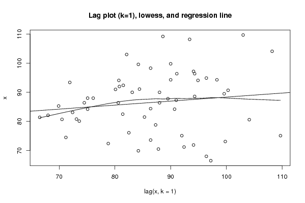
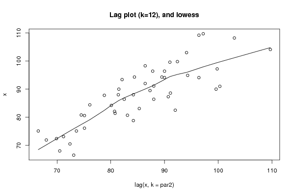
| par1 = 0 ; par2 = 12 ; | |||||||||||||||||||||||||||||||||||||||||||||||||||||
| Parameters (R input): | |||||||||||||||||||||||||||||||||||||||||||||||||||||
| par1 = 0 ; par2 = 12 ; | |||||||||||||||||||||||||||||||||||||||||||||||||||||
| R code (references can be found in the software module): | |||||||||||||||||||||||||||||||||||||||||||||||||||||
par1 <- as.numeric(par1) | |||||||||||||||||||||||||||||||||||||||||||||||||||||