Free Statistics
of Irreproducible Research!
Description of Statistical Computation | |||||||||||||||||||||||||||||||||
|---|---|---|---|---|---|---|---|---|---|---|---|---|---|---|---|---|---|---|---|---|---|---|---|---|---|---|---|---|---|---|---|---|---|
| Author's title | |||||||||||||||||||||||||||||||||
| Author | *Unverified author* | ||||||||||||||||||||||||||||||||
| R Software Module | rwasp_density.wasp | ||||||||||||||||||||||||||||||||
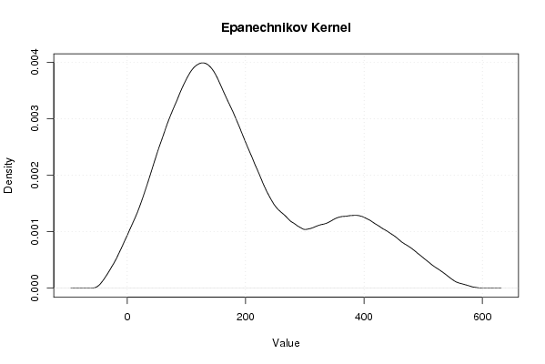
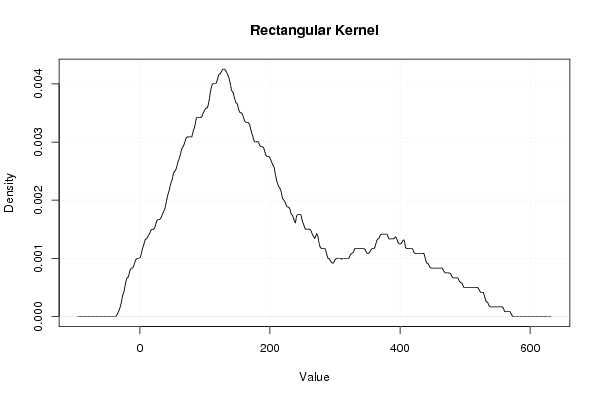
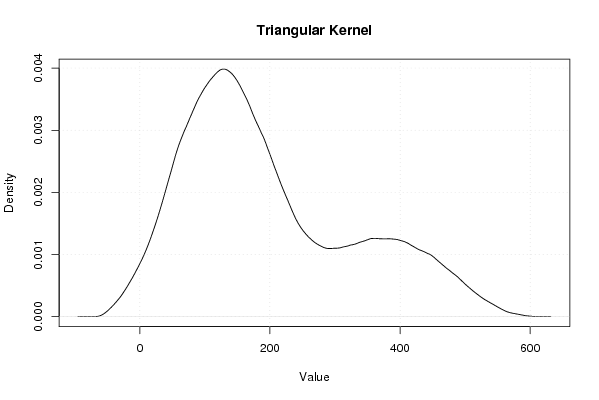
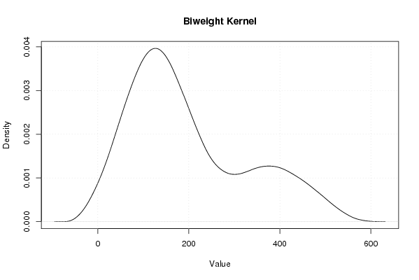
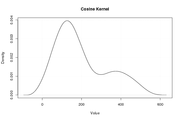
| Title produced by software | Kernel Density Estimation | ||||||||||||||||||||||||||||||||
| Date of computation | Sun, 15 Feb 2009 14:46:29 -0700 | ||||||||||||||||||||||||||||||||
| Cite this page as follows | Statistical Computations at FreeStatistics.org, Office for Research Development and Education, URL https://freestatistics.org/blog/index.php?v=date/2009/Feb/15/t1234734623vusadfildjxk8v2.htm/, Retrieved Wed, 02 Jul 2025 03:31:12 +0000 | ||||||||||||||||||||||||||||||||
| Statistical Computations at FreeStatistics.org, Office for Research Development and Education, URL https://freestatistics.org/blog/index.php?pk=37601, Retrieved Wed, 02 Jul 2025 03:31:12 +0000 | |||||||||||||||||||||||||||||||||
| QR Codes: | |||||||||||||||||||||||||||||||||
|
| |||||||||||||||||||||||||||||||||
| Original text written by user: | |||||||||||||||||||||||||||||||||
| IsPrivate? | No (this computation is public) | ||||||||||||||||||||||||||||||||
| User-defined keywords | |||||||||||||||||||||||||||||||||
| Estimated Impact | 254 | ||||||||||||||||||||||||||||||||
Tree of Dependent Computations | |||||||||||||||||||||||||||||||||
| Family? (F = Feedback message, R = changed R code, M = changed R Module, P = changed Parameters, D = changed Data) | |||||||||||||||||||||||||||||||||
| - [Univariate Data Series] [BNP USA 1889-1960] [2009-02-15 14:00:36] [74be16979710d4c4e7c6647856088456] - RMP [Histogram] [] [2009-02-15 21:36:45] [74be16979710d4c4e7c6647856088456] - RMP [Kernel Density Estimation] [] [2009-02-15 21:46:29] [d41d8cd98f00b204e9800998ecf8427e] [Current] - [Kernel Density Estimation] [Dichtheidsgrafiek...] [2009-02-16 07:26:59] [74be16979710d4c4e7c6647856088456] - PD [Kernel Density Estimation] [Duncan Huysmans O...] [2009-06-05 21:26:48] [3ccda03dddd60e52bd63ea4afd424344] - RMPD [Quartiles] [Opgave 3 opdracht...] [2009-06-05 21:34:48] [3ccda03dddd60e52bd63ea4afd424344] - RMPD [Notched Boxplots] [Duncan Huysmans O...] [2009-06-05 21:42:30] [3ccda03dddd60e52bd63ea4afd424344] - RMP [Harrell-Davis Quantiles] [Duncan Huysmans O...] [2009-06-05 22:08:50] [3ccda03dddd60e52bd63ea4afd424344] - RMP [Harrell-Davis Quantiles] [Duncan Huysmans O...] [2009-06-05 22:15:49] [3ccda03dddd60e52bd63ea4afd424344] | |||||||||||||||||||||||||||||||||
| Feedback Forum | |||||||||||||||||||||||||||||||||
Post a new message | |||||||||||||||||||||||||||||||||
Dataset | |||||||||||||||||||||||||||||||||
| Dataseries X: | |||||||||||||||||||||||||||||||||
49.1 52.7 55.1 60.4 57.5 55.9 62.6 61.3 67.1 68.6 74.8 76.9 85.7 86.5 90.8 89.7 96.3 107.5 109.2 100.2 116.8 120.1 123.3 130.2 131.4 125.6 124.5 134.3 135.2 151.8 146.4 140.0 127.8 148.0 165.9 165.5 179.9 190.0 189.8 190.9 203.6 183.5 169.3 144.2 141.5 154.3 169.5 194.0 203.2 192.9 209.4 227.2 263.7 297.8 337.1 361.3 355.2 312.6 309.9 323.7 324.1 355.3 383.4 395.1 412.8 407.0 438.0 446.1 452.5 447.3 475.9 487.7 | |||||||||||||||||||||||||||||||||
Tables (Output of Computation) | |||||||||||||||||||||||||||||||||
| |||||||||||||||||||||||||||||||||
Figures (Output of Computation) | |||||||||||||||||||||||||||||||||
Input Parameters & R Code | |||||||||||||||||||||||||||||||||
| Parameters (Session): | |||||||||||||||||||||||||||||||||
| par1 = 0 ; | |||||||||||||||||||||||||||||||||
| Parameters (R input): | |||||||||||||||||||||||||||||||||
| par1 = 0 ; | |||||||||||||||||||||||||||||||||
| R code (references can be found in the software module): | |||||||||||||||||||||||||||||||||
if (par1 == '0') bw <- 'nrd0' | |||||||||||||||||||||||||||||||||