Free Statistics
of Irreproducible Research!
Description of Statistical Computation | |||||||||||||||||||||||||||||||||
|---|---|---|---|---|---|---|---|---|---|---|---|---|---|---|---|---|---|---|---|---|---|---|---|---|---|---|---|---|---|---|---|---|---|
| Author's title | |||||||||||||||||||||||||||||||||
| Author | *Unverified author* | ||||||||||||||||||||||||||||||||
| R Software Module | rwasp_density.wasp | ||||||||||||||||||||||||||||||||
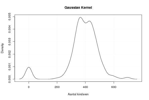
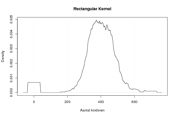
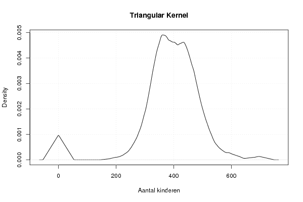
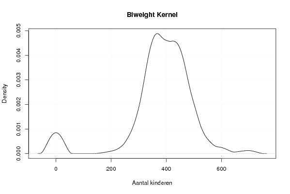
| Title produced by software | Kernel Density Estimation | ||||||||||||||||||||||||||||||||
| Date of computation | Sun, 15 Feb 2009 14:54:16 -0700 | ||||||||||||||||||||||||||||||||
| Cite this page as follows | Statistical Computations at FreeStatistics.org, Office for Research Development and Education, URL https://freestatistics.org/blog/index.php?v=date/2009/Feb/15/t1234734930yta6ecqo9f9hxsn.htm/, Retrieved Sat, 11 May 2024 14:45:19 +0000 | ||||||||||||||||||||||||||||||||
| Statistical Computations at FreeStatistics.org, Office for Research Development and Education, URL https://freestatistics.org/blog/index.php?pk=37602, Retrieved Sat, 11 May 2024 14:45:19 +0000 | |||||||||||||||||||||||||||||||||
| QR Codes: | |||||||||||||||||||||||||||||||||
|
| |||||||||||||||||||||||||||||||||
| Original text written by user: | |||||||||||||||||||||||||||||||||
| IsPrivate? | No (this computation is public) | ||||||||||||||||||||||||||||||||
| User-defined keywords | |||||||||||||||||||||||||||||||||
| Estimated Impact | 192 | ||||||||||||||||||||||||||||||||
Tree of Dependent Computations | |||||||||||||||||||||||||||||||||
| Family? (F = Feedback message, R = changed R code, M = changed R Module, P = changed Parameters, D = changed Data) | |||||||||||||||||||||||||||||||||
| - [Kernel Density Estimation] [Dichtheidsgrafiek...] [2009-02-15 21:54:16] [d41d8cd98f00b204e9800998ecf8427e] [Current] - [Kernel Density Estimation] [Gabriels Wim Dich...] [2009-02-28 14:07:14] [74be16979710d4c4e7c6647856088456] - RMPD [Notched Boxplots] [Gabriels Wim Boxp...] [2009-02-28 14:21:52] [74be16979710d4c4e7c6647856088456] - RMPD [Notched Boxplots] [Gabriels Wim Boxp...] [2009-02-28 14:37:15] [74be16979710d4c4e7c6647856088456] | |||||||||||||||||||||||||||||||||
| Feedback Forum | |||||||||||||||||||||||||||||||||
Post a new message | |||||||||||||||||||||||||||||||||
Dataset | |||||||||||||||||||||||||||||||||
| Dataseries X: | |||||||||||||||||||||||||||||||||
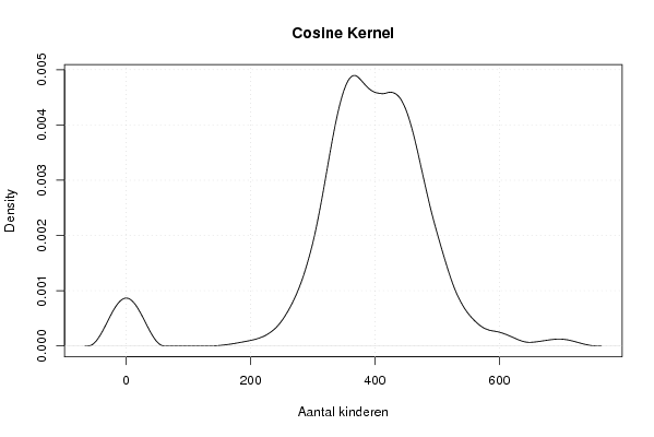
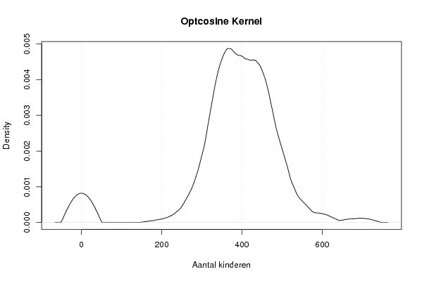
374 572 402 589 507 628 698 451 694 0 488 526 343 494 447 0 470 366 517 483 485 530 308 481 437 468 502 408 479 436 410 451 344 411 0 427 454 365 499 416 430 470 325 452 442 488 446 523 594 439 588 503 444 525 375 472 436 458 514 0 472 360 450 549 361 466 387 457 470 396 471 422 404 414 342 459 379 0 410 319 411 371 365 429 333 392 469 432 534 379 436 448 358 492 387 529 475 439 459 361 0 0 394 425 341 455 403 471 523 389 531 468 398 446 355 435 353 0 400 332 389 355 384 406 356 336 351 278 265 229 387 435 317 490 472 440 429 350 489 494 436 436 375 429 0 434 472 362 440 433 400 442 316 432 401 434 488 377 484 377 0 0 300 389 337 376 377 331 339 356 280 249 196 268 379 401 404 397 419 421 407 296 468 475 422 456 339 446 419 346 327 326 403 359 358 421 322 367 394 356 418 344 372 358 373 379 0 348 369 341 390 279 325 354 346 358 296 356 337 360 474 362 440 443 435 429 341 434 329 416 430 307 408 322 0 324 303 369 328 258 372 298 376 306 359 418 311 355 335 345 318 291 340 0 356 419 296 361 371 392 383 286 362 358 | |||||||||||||||||||||||||||||||||
Tables (Output of Computation) | |||||||||||||||||||||||||||||||||
| |||||||||||||||||||||||||||||||||
Figures (Output of Computation) | |||||||||||||||||||||||||||||||||
Input Parameters & R Code | |||||||||||||||||||||||||||||||||
| Parameters (Session): | |||||||||||||||||||||||||||||||||
| par1 = 0 ; | |||||||||||||||||||||||||||||||||
| Parameters (R input): | |||||||||||||||||||||||||||||||||
| par1 = 0 ; | |||||||||||||||||||||||||||||||||
| R code (references can be found in the software module): | |||||||||||||||||||||||||||||||||
if (par1 == '0') bw <- 'nrd0' | |||||||||||||||||||||||||||||||||