Free Statistics
of Irreproducible Research!
Description of Statistical Computation | |||||||||||||||||||||||||||||||||||||||||||||
|---|---|---|---|---|---|---|---|---|---|---|---|---|---|---|---|---|---|---|---|---|---|---|---|---|---|---|---|---|---|---|---|---|---|---|---|---|---|---|---|---|---|---|---|---|---|
| Author's title | |||||||||||||||||||||||||||||||||||||||||||||
| Author | *The author of this computation has been verified* | ||||||||||||||||||||||||||||||||||||||||||||
| R Software Module | rwasp_regression_trees1.wasp | ||||||||||||||||||||||||||||||||||||||||||||
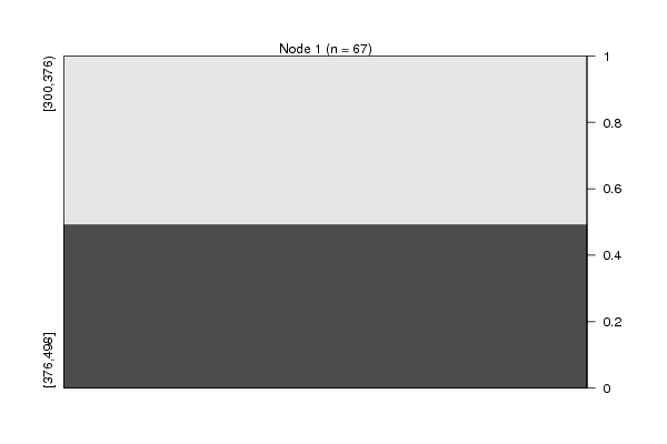
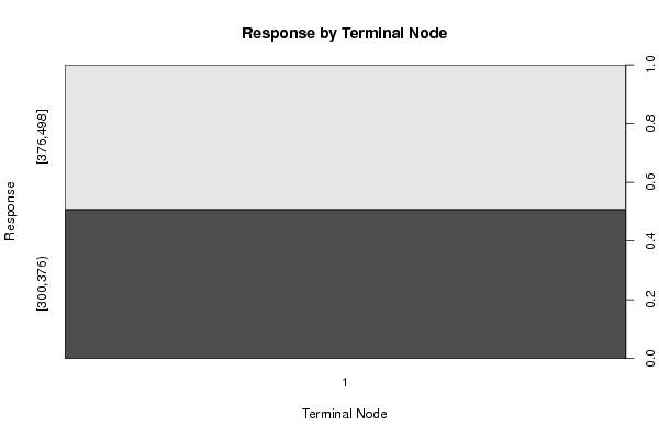
| Title produced by software | Recursive Partitioning (Regression Trees) | ||||||||||||||||||||||||||||||||||||||||||||
| Date of computation | Tue, 21 Dec 2010 14:33:56 +0000 | ||||||||||||||||||||||||||||||||||||||||||||
| Cite this page as follows | Statistical Computations at FreeStatistics.org, Office for Research Development and Education, URL https://freestatistics.org/blog/index.php?v=date/2010/Dec/21/t1292942466vnapvluuj0kidp4.htm/, Retrieved Sun, 06 Jul 2025 08:59:56 +0000 | ||||||||||||||||||||||||||||||||||||||||||||
| Statistical Computations at FreeStatistics.org, Office for Research Development and Education, URL https://freestatistics.org/blog/index.php?pk=113626, Retrieved Sun, 06 Jul 2025 08:59:56 +0000 | |||||||||||||||||||||||||||||||||||||||||||||
| QR Codes: | |||||||||||||||||||||||||||||||||||||||||||||
|
| |||||||||||||||||||||||||||||||||||||||||||||
| Original text written by user: | |||||||||||||||||||||||||||||||||||||||||||||
| IsPrivate? | No (this computation is public) | ||||||||||||||||||||||||||||||||||||||||||||
| User-defined keywords | |||||||||||||||||||||||||||||||||||||||||||||
| Estimated Impact | 257 | ||||||||||||||||||||||||||||||||||||||||||||
Tree of Dependent Computations | |||||||||||||||||||||||||||||||||||||||||||||
| Family? (F = Feedback message, R = changed R code, M = changed R Module, P = changed Parameters, D = changed Data) | |||||||||||||||||||||||||||||||||||||||||||||
| - [Recursive Partitioning (Regression Trees)] [] [2010-12-05 18:59:57] [b98453cac15ba1066b407e146608df68] - PD [Recursive Partitioning (Regression Trees)] [WS 10 - recursive...] [2010-12-11 16:07:41] [033eb2749a430605d9b2be7c4aac4a0c] - P [Recursive Partitioning (Regression Trees)] [WS 10 - recursive...] [2010-12-11 16:27:23] [033eb2749a430605d9b2be7c4aac4a0c] - P [Recursive Partitioning (Regression Trees)] [] [2010-12-13 18:26:49] [d7b28a0391ab3b2ddc9f9fba95a43f33] - PD [Recursive Partitioning (Regression Trees)] [] [2010-12-21 14:33:56] [44163a3390d803b6e1dc8c2f0815c192] [Current] | |||||||||||||||||||||||||||||||||||||||||||||
| Feedback Forum | |||||||||||||||||||||||||||||||||||||||||||||
Post a new message | |||||||||||||||||||||||||||||||||||||||||||||
Dataset | |||||||||||||||||||||||||||||||||||||||||||||
| Dataseries X: | |||||||||||||||||||||||||||||||||||||||||||||
300 2.26 591.000 302 2.57 589.000 400 3.07 584.000 392 2.76 573.000 373 2.51 567.000 379 2.87 569.000 303 3.14 621.000 324 3.11 629.000 353 3.16 628.000 392 2.47 612.000 327 2.57 595.000 376 2.89 597.000 329 2.63 593.000 359 2.38 590.000 413 1.69 580.000 338 1.96 574.000 422 2.19 573.000 390 1.87 573.000 370 1.60 620.000 367 1.63 626.000 406 1.22 620.000 418 1.21 588.000 346 1.49 566.000 350 1.64 557.000 330 1.66 561.000 318 1.77 549.000 382 1.82 532.000 337 1.78 526.000 372 1.28 511.000 422 1.29 499.000 428 1.37 555.000 426 1.12 565.000 396 1.51 542.000 458 2.24 527.000 315 2.94 510.000 337 3.09 514.000 386 3.46 517.000 352 3.64 508.000 383 4.39 493.000 439 4.15 490.000 397 5.21 469.000 453 5.80 478.000 363 5.91 528.000 365 5.39 534.000 474 5.46 518.000 373 4.72 506.000 403 3.14 502.000 384 2.63 516.000 364 2.32 528.000 361 1.93 533.000 419 0.62 536.000 352 0.60 537.000 363 -0.37 524.000 410 -1.10 536.000 361 -1.68 587.000 383 -0.78 597.000 342 -1.19 581.000 369 -0.79 564.000 361 -0.12 558.000 317 0.26 575.000 386 0.62 580.000 318 0.70 575.000 407 1.66 563.000 393 1.80 552.000 404 2.27 537.000 498 2.46 545.000 438 2.57 601.000 | |||||||||||||||||||||||||||||||||||||||||||||
Tables (Output of Computation) | |||||||||||||||||||||||||||||||||||||||||||||
| |||||||||||||||||||||||||||||||||||||||||||||
Figures (Output of Computation) | |||||||||||||||||||||||||||||||||||||||||||||
Input Parameters & R Code | |||||||||||||||||||||||||||||||||||||||||||||
| Parameters (Session): | |||||||||||||||||||||||||||||||||||||||||||||
| par1 = 1 ; par2 = quantiles ; par3 = 3 ; par4 = no ; | |||||||||||||||||||||||||||||||||||||||||||||
| Parameters (R input): | |||||||||||||||||||||||||||||||||||||||||||||
| par1 = 1 ; par2 = quantiles ; par3 = 2 ; par4 = no ; | |||||||||||||||||||||||||||||||||||||||||||||
| R code (references can be found in the software module): | |||||||||||||||||||||||||||||||||||||||||||||
library(party) | |||||||||||||||||||||||||||||||||||||||||||||