Repository of Reproducible Computations

Free Statistics

of Irreproducible Research!

Author's title

Author

*Unverified author*

R Software Module

rwasp_autocorrelation.wasp

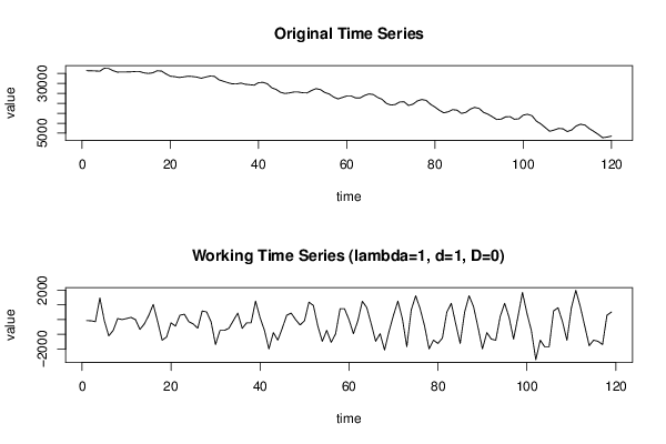
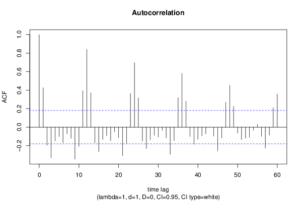
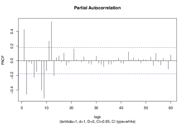
Title produced by software

(Partial) Autocorrelation Function

Date of computation

Mon, 12 Aug 2013 10:00:03 -0400

Cite this page as follows

Statistical Computations at FreeStatistics.org, Office for Research Development and Education, URL https://freestatistics.org/blog/index.php?v=date/2013/Aug/12/t1376316048eo9jiqcwd0wq5xi.htm/, Retrieved Sun, 28 Apr 2024 08:53:08 +0000

Statistical Computations at FreeStatistics.org, Office for Research Development and Education, URL https://freestatistics.org/blog/index.php?pk=211035, Retrieved Sun, 28 Apr 2024 08:53:08 +0000

QR Codes:

Paste this QR Code to cite your computation.

Original text written by user:

IsPrivate?

No (this computation is public)

User-defined keywords

Anthony Van Dyck

Estimated Impact

142

Family? (F = Feedback message, R = changed R code, M = changed R Module, P = changed Parameters, D = changed Data)

-     [Univariate Data Series] [Tijdreeks 1 - stap 2] [2013-08-12 11:07:04] [c4bfab449d963e708b9482b0c0d301bf]
-   P   [Univariate Data Series] [Tijdreeks A - Stap 2] [2013-08-12 11:17:51] [fffbdc2eb6bf36a612a50d50ad291a0a]
- RMP     [Histogram] [Tijdreeks A - Stap 3] [2013-08-12 11:22:38] [fffbdc2eb6bf36a612a50d50ad291a0a]
- R P       [Histogram] [Tijdreeks A -stap 5] [2013-08-12 11:38:26] [c4bfab449d963e708b9482b0c0d301bf]
-   P         [Histogram] [Tijdreeks A -stap 5] [2013-08-12 11:42:06] [c4bfab449d963e708b9482b0c0d301bf]
- RMP           [Harrell-Davis Quantiles] [Tijdreeks A - sta...] [2013-08-12 12:35:57] [fffbdc2eb6bf36a612a50d50ad291a0a]
- R P             [Harrell-Davis Quantiles] [Tijdreeks A - sta...] [2013-08-12 12:48:29] [c4bfab449d963e708b9482b0c0d301bf]
- RMP               [(Partial) Autocorrelation Function] [Tijdreeks A - sta...] [2013-08-12 13:54:06] [fffbdc2eb6bf36a612a50d50ad291a0a]
- R                     [(Partial) Autocorrelation Function] [Tijdreeks A - sta...] [2013-08-12 14:00:03] [946b987ea445738c2c70467dba74cc4f] [Current]

Feedback Forum

Post a new message

Dataseries X:

Download CSV

Histogram

Boxplots

Summary of computational transaction
Raw Input	view raw input (R code)
Raw Output	view raw output of R engine
Computing time	5 seconds
R Server	'Gwilym Jenkins' @ jenkins.wessa.net

\begin{tabular}{lllllllll}
\hline
Summary of computational transaction \tabularnewline
Raw Input & view raw input (R code)  \tabularnewline
Raw Output & view raw output of R engine  \tabularnewline
Computing time & 5 seconds \tabularnewline
R Server & 'Gwilym Jenkins' @ jenkins.wessa.net \tabularnewline
\hline
\end{tabular}
%Source: https://freestatistics.org/blog/index.php?pk=211035&T=0

[TABLE]
[ROW][C]Summary of computational transaction[/C][/ROW]
[ROW][C]Raw Input[/C][C]view raw input (R code) [/C][/ROW]
[ROW][C]Raw Output[/C][C]view raw output of R engine [/C][/ROW]
[ROW][C]Computing time[/C][C]5 seconds[/C][/ROW]
[ROW][C]R Server[/C][C]'Gwilym Jenkins' @ jenkins.wessa.net[/C][/ROW]
[/TABLE]
Source: https://freestatistics.org/blog/index.php?pk=211035&T=0

Globally Unique Identifier (entire table): ba.freestatistics.org/blog/index.php?pk=211035&T=0

As an alternative you can also use a QR Code:

The GUIDs for individual cells are displayed in the table below:

Summary of computational transaction
Raw Input	view raw input (R code)
Raw Output	view raw output of R engine
Computing time	5 seconds
R Server	'Gwilym Jenkins' @ jenkins.wessa.net

Autocorrelation Function
Time lag k	ACF(k)	T-STAT	P-value
1	0.426075	4.6479	4e-06
2	-0.195502	-2.1327	0.017503
3	-0.33047	-3.605	0.000229
4	-0.149182	-1.6274	0.05315
5	-0.102227	-1.1152	0.133514
6	-0.16621	-1.8131	0.036166
7	-0.071816	-0.7834	0.217468
8	-0.121614	-1.3267	0.093582
9	-0.345624	-3.7703	0.000128
10	-0.207873	-2.2676	0.012578
11	0.393578	4.2934	1.8e-05
12	0.840833	9.1724	0
13	0.370614	4.0429	4.7e-05
14	-0.1696	-1.8501	0.033389
15	-0.265177	-2.8927	0.002271
16	-0.13474	-1.4698	0.072122
17	-0.09172	-1.0005	0.159539
18	-0.146346	-1.5964	0.056521
19	-0.050391	-0.5497	0.291778
20	-0.114032	-1.2439	0.107984
21	-0.307547	-3.3549	0.000533
22	-0.172876	-1.8859	0.030876
23	0.363259	3.9627	6.3e-05
24	0.697058	7.604	0
25	0.316972	3.4578	0.000378
26	-0.148585	-1.6209	0.053846
27	-0.231381	-2.5241	0.006459
28	-0.13706	-1.4951	0.068762
29	-0.089296	-0.9741	0.165991
30	-0.106971	-1.1669	0.122789
31	-0.035667	-0.3891	0.348954
32	-0.116846	-1.2746	0.10246
33	-0.293036	-3.1966	0.00089
34	-0.144951	-1.5812	0.05824
35	0.319135	3.4814	0.000349
36	0.579855	6.3255	0
37	0.280789	3.063	0.001355
38	-0.101997	-1.1127	0.13405
39	-0.184734	-2.0152	0.023068
40	-0.13215	-1.4416	0.076023
41	-0.094651	-1.0325	0.15196
42	-0.07266	-0.7926	0.214786
43	0.000528	0.0058	0.497706
44	-0.097941	-1.0684	0.14375
45	-0.25652	-2.7983	0.002997
46	-0.117863	-1.2857	0.100516
47	0.268066	2.9243	0.002067
48	0.452282	4.9338	1e-06
49	0.224297	2.4468	0.007938
50	-0.064262	-0.701	0.242331
51	-0.134749	-1.4699	0.072109
52	-0.118969	-1.2978	0.098433
53	-0.110655	-1.2071	0.114893
54	-0.034648	-0.378	0.353064
55	0.03063	0.3341	0.369434
56	-0.098888	-1.0787	0.141443
57	-0.226079	-2.4662	0.00754
58	-0.086514	-0.9438	0.173602
59	0.210396	2.2951	0.011738
60	0.357368	3.8984	8e-05

\begin{tabular}{lllllllll}
\hline
Autocorrelation Function \tabularnewline
Time lag k & ACF(k) & T-STAT & P-value \tabularnewline
1 & 0.426075 & 4.6479 & 4e-06 \tabularnewline
2 & -0.195502 & -2.1327 & 0.017503 \tabularnewline
3 & -0.33047 & -3.605 & 0.000229 \tabularnewline
4 & -0.149182 & -1.6274 & 0.05315 \tabularnewline
5 & -0.102227 & -1.1152 & 0.133514 \tabularnewline
6 & -0.16621 & -1.8131 & 0.036166 \tabularnewline
7 & -0.071816 & -0.7834 & 0.217468 \tabularnewline
8 & -0.121614 & -1.3267 & 0.093582 \tabularnewline
9 & -0.345624 & -3.7703 & 0.000128 \tabularnewline
10 & -0.207873 & -2.2676 & 0.012578 \tabularnewline
11 & 0.393578 & 4.2934 & 1.8e-05 \tabularnewline
12 & 0.840833 & 9.1724 & 0 \tabularnewline
13 & 0.370614 & 4.0429 & 4.7e-05 \tabularnewline
14 & -0.1696 & -1.8501 & 0.033389 \tabularnewline
15 & -0.265177 & -2.8927 & 0.002271 \tabularnewline
16 & -0.13474 & -1.4698 & 0.072122 \tabularnewline
17 & -0.09172 & -1.0005 & 0.159539 \tabularnewline
18 & -0.146346 & -1.5964 & 0.056521 \tabularnewline
19 & -0.050391 & -0.5497 & 0.291778 \tabularnewline
20 & -0.114032 & -1.2439 & 0.107984 \tabularnewline
21 & -0.307547 & -3.3549 & 0.000533 \tabularnewline
22 & -0.172876 & -1.8859 & 0.030876 \tabularnewline
23 & 0.363259 & 3.9627 & 6.3e-05 \tabularnewline
24 & 0.697058 & 7.604 & 0 \tabularnewline
25 & 0.316972 & 3.4578 & 0.000378 \tabularnewline
26 & -0.148585 & -1.6209 & 0.053846 \tabularnewline
27 & -0.231381 & -2.5241 & 0.006459 \tabularnewline
28 & -0.13706 & -1.4951 & 0.068762 \tabularnewline
29 & -0.089296 & -0.9741 & 0.165991 \tabularnewline
30 & -0.106971 & -1.1669 & 0.122789 \tabularnewline
31 & -0.035667 & -0.3891 & 0.348954 \tabularnewline
32 & -0.116846 & -1.2746 & 0.10246 \tabularnewline
33 & -0.293036 & -3.1966 & 0.00089 \tabularnewline
34 & -0.144951 & -1.5812 & 0.05824 \tabularnewline
35 & 0.319135 & 3.4814 & 0.000349 \tabularnewline
36 & 0.579855 & 6.3255 & 0 \tabularnewline
37 & 0.280789 & 3.063 & 0.001355 \tabularnewline
38 & -0.101997 & -1.1127 & 0.13405 \tabularnewline
39 & -0.184734 & -2.0152 & 0.023068 \tabularnewline
40 & -0.13215 & -1.4416 & 0.076023 \tabularnewline
41 & -0.094651 & -1.0325 & 0.15196 \tabularnewline
42 & -0.07266 & -0.7926 & 0.214786 \tabularnewline
43 & 0.000528 & 0.0058 & 0.497706 \tabularnewline
44 & -0.097941 & -1.0684 & 0.14375 \tabularnewline
45 & -0.25652 & -2.7983 & 0.002997 \tabularnewline
46 & -0.117863 & -1.2857 & 0.100516 \tabularnewline
47 & 0.268066 & 2.9243 & 0.002067 \tabularnewline
48 & 0.452282 & 4.9338 & 1e-06 \tabularnewline
49 & 0.224297 & 2.4468 & 0.007938 \tabularnewline
50 & -0.064262 & -0.701 & 0.242331 \tabularnewline
51 & -0.134749 & -1.4699 & 0.072109 \tabularnewline
52 & -0.118969 & -1.2978 & 0.098433 \tabularnewline
53 & -0.110655 & -1.2071 & 0.114893 \tabularnewline
54 & -0.034648 & -0.378 & 0.353064 \tabularnewline
55 & 0.03063 & 0.3341 & 0.369434 \tabularnewline
56 & -0.098888 & -1.0787 & 0.141443 \tabularnewline
57 & -0.226079 & -2.4662 & 0.00754 \tabularnewline
58 & -0.086514 & -0.9438 & 0.173602 \tabularnewline
59 & 0.210396 & 2.2951 & 0.011738 \tabularnewline
60 & 0.357368 & 3.8984 & 8e-05 \tabularnewline
\hline
\end{tabular}
%Source: https://freestatistics.org/blog/index.php?pk=211035&T=1

[TABLE]
[ROW][C]Autocorrelation Function[/C][/ROW]
[ROW][C]Time lag k[/C][C]ACF(k)[/C][C]T-STAT[/C][C]P-value[/C][/ROW]
[ROW][C]1[/C][C]0.426075[/C][C]4.6479[/C][C]4e-06[/C][/ROW]
[ROW][C]2[/C][C]-0.195502[/C][C]-2.1327[/C][C]0.017503[/C][/ROW]
[ROW][C]3[/C][C]-0.33047[/C][C]-3.605[/C][C]0.000229[/C][/ROW]
[ROW][C]4[/C][C]-0.149182[/C][C]-1.6274[/C][C]0.05315[/C][/ROW]
[ROW][C]5[/C][C]-0.102227[/C][C]-1.1152[/C][C]0.133514[/C][/ROW]
[ROW][C]6[/C][C]-0.16621[/C][C]-1.8131[/C][C]0.036166[/C][/ROW]
[ROW][C]7[/C][C]-0.071816[/C][C]-0.7834[/C][C]0.217468[/C][/ROW]
[ROW][C]8[/C][C]-0.121614[/C][C]-1.3267[/C][C]0.093582[/C][/ROW]
[ROW][C]9[/C][C]-0.345624[/C][C]-3.7703[/C][C]0.000128[/C][/ROW]
[ROW][C]10[/C][C]-0.207873[/C][C]-2.2676[/C][C]0.012578[/C][/ROW]
[ROW][C]11[/C][C]0.393578[/C][C]4.2934[/C][C]1.8e-05[/C][/ROW]
[ROW][C]12[/C][C]0.840833[/C][C]9.1724[/C][C]0[/C][/ROW]
[ROW][C]13[/C][C]0.370614[/C][C]4.0429[/C][C]4.7e-05[/C][/ROW]
[ROW][C]14[/C][C]-0.1696[/C][C]-1.8501[/C][C]0.033389[/C][/ROW]
[ROW][C]15[/C][C]-0.265177[/C][C]-2.8927[/C][C]0.002271[/C][/ROW]
[ROW][C]16[/C][C]-0.13474[/C][C]-1.4698[/C][C]0.072122[/C][/ROW]
[ROW][C]17[/C][C]-0.09172[/C][C]-1.0005[/C][C]0.159539[/C][/ROW]
[ROW][C]18[/C][C]-0.146346[/C][C]-1.5964[/C][C]0.056521[/C][/ROW]
[ROW][C]19[/C][C]-0.050391[/C][C]-0.5497[/C][C]0.291778[/C][/ROW]
[ROW][C]20[/C][C]-0.114032[/C][C]-1.2439[/C][C]0.107984[/C][/ROW]
[ROW][C]21[/C][C]-0.307547[/C][C]-3.3549[/C][C]0.000533[/C][/ROW]
[ROW][C]22[/C][C]-0.172876[/C][C]-1.8859[/C][C]0.030876[/C][/ROW]
[ROW][C]23[/C][C]0.363259[/C][C]3.9627[/C][C]6.3e-05[/C][/ROW]
[ROW][C]24[/C][C]0.697058[/C][C]7.604[/C][C]0[/C][/ROW]
[ROW][C]25[/C][C]0.316972[/C][C]3.4578[/C][C]0.000378[/C][/ROW]
[ROW][C]26[/C][C]-0.148585[/C][C]-1.6209[/C][C]0.053846[/C][/ROW]
[ROW][C]27[/C][C]-0.231381[/C][C]-2.5241[/C][C]0.006459[/C][/ROW]
[ROW][C]28[/C][C]-0.13706[/C][C]-1.4951[/C][C]0.068762[/C][/ROW]
[ROW][C]29[/C][C]-0.089296[/C][C]-0.9741[/C][C]0.165991[/C][/ROW]
[ROW][C]30[/C][C]-0.106971[/C][C]-1.1669[/C][C]0.122789[/C][/ROW]
[ROW][C]31[/C][C]-0.035667[/C][C]-0.3891[/C][C]0.348954[/C][/ROW]
[ROW][C]32[/C][C]-0.116846[/C][C]-1.2746[/C][C]0.10246[/C][/ROW]
[ROW][C]33[/C][C]-0.293036[/C][C]-3.1966[/C][C]0.00089[/C][/ROW]
[ROW][C]34[/C][C]-0.144951[/C][C]-1.5812[/C][C]0.05824[/C][/ROW]
[ROW][C]35[/C][C]0.319135[/C][C]3.4814[/C][C]0.000349[/C][/ROW]
[ROW][C]36[/C][C]0.579855[/C][C]6.3255[/C][C]0[/C][/ROW]
[ROW][C]37[/C][C]0.280789[/C][C]3.063[/C][C]0.001355[/C][/ROW]
[ROW][C]38[/C][C]-0.101997[/C][C]-1.1127[/C][C]0.13405[/C][/ROW]
[ROW][C]39[/C][C]-0.184734[/C][C]-2.0152[/C][C]0.023068[/C][/ROW]
[ROW][C]40[/C][C]-0.13215[/C][C]-1.4416[/C][C]0.076023[/C][/ROW]
[ROW][C]41[/C][C]-0.094651[/C][C]-1.0325[/C][C]0.15196[/C][/ROW]
[ROW][C]42[/C][C]-0.07266[/C][C]-0.7926[/C][C]0.214786[/C][/ROW]
[ROW][C]43[/C][C]0.000528[/C][C]0.0058[/C][C]0.497706[/C][/ROW]
[ROW][C]44[/C][C]-0.097941[/C][C]-1.0684[/C][C]0.14375[/C][/ROW]
[ROW][C]45[/C][C]-0.25652[/C][C]-2.7983[/C][C]0.002997[/C][/ROW]
[ROW][C]46[/C][C]-0.117863[/C][C]-1.2857[/C][C]0.100516[/C][/ROW]
[ROW][C]47[/C][C]0.268066[/C][C]2.9243[/C][C]0.002067[/C][/ROW]
[ROW][C]48[/C][C]0.452282[/C][C]4.9338[/C][C]1e-06[/C][/ROW]
[ROW][C]49[/C][C]0.224297[/C][C]2.4468[/C][C]0.007938[/C][/ROW]
[ROW][C]50[/C][C]-0.064262[/C][C]-0.701[/C][C]0.242331[/C][/ROW]
[ROW][C]51[/C][C]-0.134749[/C][C]-1.4699[/C][C]0.072109[/C][/ROW]
[ROW][C]52[/C][C]-0.118969[/C][C]-1.2978[/C][C]0.098433[/C][/ROW]
[ROW][C]53[/C][C]-0.110655[/C][C]-1.2071[/C][C]0.114893[/C][/ROW]
[ROW][C]54[/C][C]-0.034648[/C][C]-0.378[/C][C]0.353064[/C][/ROW]
[ROW][C]55[/C][C]0.03063[/C][C]0.3341[/C][C]0.369434[/C][/ROW]
[ROW][C]56[/C][C]-0.098888[/C][C]-1.0787[/C][C]0.141443[/C][/ROW]
[ROW][C]57[/C][C]-0.226079[/C][C]-2.4662[/C][C]0.00754[/C][/ROW]
[ROW][C]58[/C][C]-0.086514[/C][C]-0.9438[/C][C]0.173602[/C][/ROW]
[ROW][C]59[/C][C]0.210396[/C][C]2.2951[/C][C]0.011738[/C][/ROW]
[ROW][C]60[/C][C]0.357368[/C][C]3.8984[/C][C]8e-05[/C][/ROW]
[/TABLE]
Source: https://freestatistics.org/blog/index.php?pk=211035&T=1

Globally Unique Identifier (entire table): ba.freestatistics.org/blog/index.php?pk=211035&T=1

As an alternative you can also use a QR Code:

The GUIDs for individual cells are displayed in the table below:

Autocorrelation Function
Time lag k	ACF(k)	T-STAT	P-value
1	0.426075	4.6479	4e-06
2	-0.195502	-2.1327	0.017503
3	-0.33047	-3.605	0.000229
4	-0.149182	-1.6274	0.05315
5	-0.102227	-1.1152	0.133514
6	-0.16621	-1.8131	0.036166
7	-0.071816	-0.7834	0.217468
8	-0.121614	-1.3267	0.093582
9	-0.345624	-3.7703	0.000128
10	-0.207873	-2.2676	0.012578
11	0.393578	4.2934	1.8e-05
12	0.840833	9.1724	0
13	0.370614	4.0429	4.7e-05
14	-0.1696	-1.8501	0.033389
15	-0.265177	-2.8927	0.002271
16	-0.13474	-1.4698	0.072122
17	-0.09172	-1.0005	0.159539
18	-0.146346	-1.5964	0.056521
19	-0.050391	-0.5497	0.291778
20	-0.114032	-1.2439	0.107984
21	-0.307547	-3.3549	0.000533
22	-0.172876	-1.8859	0.030876
23	0.363259	3.9627	6.3e-05
24	0.697058	7.604	0
25	0.316972	3.4578	0.000378
26	-0.148585	-1.6209	0.053846
27	-0.231381	-2.5241	0.006459
28	-0.13706	-1.4951	0.068762
29	-0.089296	-0.9741	0.165991
30	-0.106971	-1.1669	0.122789
31	-0.035667	-0.3891	0.348954
32	-0.116846	-1.2746	0.10246
33	-0.293036	-3.1966	0.00089
34	-0.144951	-1.5812	0.05824
35	0.319135	3.4814	0.000349
36	0.579855	6.3255	0
37	0.280789	3.063	0.001355
38	-0.101997	-1.1127	0.13405
39	-0.184734	-2.0152	0.023068
40	-0.13215	-1.4416	0.076023
41	-0.094651	-1.0325	0.15196
42	-0.07266	-0.7926	0.214786
43	0.000528	0.0058	0.497706
44	-0.097941	-1.0684	0.14375
45	-0.25652	-2.7983	0.002997
46	-0.117863	-1.2857	0.100516
47	0.268066	2.9243	0.002067
48	0.452282	4.9338	1e-06
49	0.224297	2.4468	0.007938
50	-0.064262	-0.701	0.242331
51	-0.134749	-1.4699	0.072109
52	-0.118969	-1.2978	0.098433
53	-0.110655	-1.2071	0.114893
54	-0.034648	-0.378	0.353064
55	0.03063	0.3341	0.369434
56	-0.098888	-1.0787	0.141443
57	-0.226079	-2.4662	0.00754
58	-0.086514	-0.9438	0.173602
59	0.210396	2.2951	0.011738
60	0.357368	3.8984	8e-05

Partial Autocorrelation Function
Time lag k	PACF(k)	T-STAT	P-value
1	0.426075	4.6479	4e-06
2	-0.460672	-5.0253	1e-06
3	-0.019414	-0.2118	0.416319
4	-0.040179	-0.4383	0.330982
5	-0.228276	-2.4902	0.007074
6	-0.14866	-1.6217	0.053758
7	0.009637	0.1051	0.458224
8	-0.404232	-4.4096	1.1e-05
9	-0.511257	-5.5772	0
10	-0.137243	-1.4971	0.068502
11	0.266971	2.9123	0.002143
12	0.53628	5.8501	0
13	-0.206395	-2.2515	0.013094
14	0.042461	0.4632	0.322035
15	0.064533	0.704	0.241412
16	-0.015032	-0.164	0.435012
17	0.104182	1.1365	0.129017
18	-0.063398	-0.6916	0.245272
19	-0.023349	-0.2547	0.399695
20	-0.001787	-0.0195	0.492238
21	0.162408	1.7717	0.039505
22	0.012033	0.1313	0.447893
23	8e-05	9e-04	0.499651
24	-0.018086	-0.1973	0.421968
25	0.054029	0.5894	0.278358
26	0.001611	0.0176	0.493004
27	-0.038457	-0.4195	0.337796
28	-0.050664	-0.5527	0.290758
29	9.2e-05	0.001	0.4996
30	0.063996	0.6981	0.243235
31	-0.035972	-0.3924	0.34773
32	-0.051013	-0.5565	0.289461
33	-0.080672	-0.88	0.19031
34	0.003654	0.0399	0.484134
35	-0.048949	-0.534	0.297177
36	-0.048333	-0.5272	0.299501
37	-0.013435	-0.1466	0.441864
38	0.008863	0.0967	0.461571
39	0.039226	0.4279	0.334747
40	-0.032076	-0.3499	0.363515
41	-0.041626	-0.4541	0.325296
42	-0.003106	-0.0339	0.486514
43	0.12128	1.323	0.094185
44	0.012903	0.1408	0.444151
45	0.042117	0.4594	0.323378
46	0.007901	0.0862	0.465728
47	0.022376	0.2441	0.403787
48	-0.031575	-0.3444	0.365561
49	0.015953	0.174	0.431068
50	0.014832	0.1618	0.435871
51	0.005924	0.0646	0.474291
52	0.050648	0.5525	0.290821
53	-0.067662	-0.7381	0.230952
54	0.100832	1.0999	0.136789
55	-0.01414	-0.1543	0.438836
56	-0.060667	-0.6618	0.254688
57	0.032976	0.3597	0.359846
58	-0.004103	-0.0448	0.482189
59	-0.115287	-1.2576	0.105493
60	0.078758	0.8591	0.195994

\begin{tabular}{lllllllll}
\hline
Partial Autocorrelation Function \tabularnewline
Time lag k & PACF(k) & T-STAT & P-value \tabularnewline
1 & 0.426075 & 4.6479 & 4e-06 \tabularnewline
2 & -0.460672 & -5.0253 & 1e-06 \tabularnewline
3 & -0.019414 & -0.2118 & 0.416319 \tabularnewline
4 & -0.040179 & -0.4383 & 0.330982 \tabularnewline
5 & -0.228276 & -2.4902 & 0.007074 \tabularnewline
6 & -0.14866 & -1.6217 & 0.053758 \tabularnewline
7 & 0.009637 & 0.1051 & 0.458224 \tabularnewline
8 & -0.404232 & -4.4096 & 1.1e-05 \tabularnewline
9 & -0.511257 & -5.5772 & 0 \tabularnewline
10 & -0.137243 & -1.4971 & 0.068502 \tabularnewline
11 & 0.266971 & 2.9123 & 0.002143 \tabularnewline
12 & 0.53628 & 5.8501 & 0 \tabularnewline
13 & -0.206395 & -2.2515 & 0.013094 \tabularnewline
14 & 0.042461 & 0.4632 & 0.322035 \tabularnewline
15 & 0.064533 & 0.704 & 0.241412 \tabularnewline
16 & -0.015032 & -0.164 & 0.435012 \tabularnewline
17 & 0.104182 & 1.1365 & 0.129017 \tabularnewline
18 & -0.063398 & -0.6916 & 0.245272 \tabularnewline
19 & -0.023349 & -0.2547 & 0.399695 \tabularnewline
20 & -0.001787 & -0.0195 & 0.492238 \tabularnewline
21 & 0.162408 & 1.7717 & 0.039505 \tabularnewline
22 & 0.012033 & 0.1313 & 0.447893 \tabularnewline
23 & 8e-05 & 9e-04 & 0.499651 \tabularnewline
24 & -0.018086 & -0.1973 & 0.421968 \tabularnewline
25 & 0.054029 & 0.5894 & 0.278358 \tabularnewline
26 & 0.001611 & 0.0176 & 0.493004 \tabularnewline
27 & -0.038457 & -0.4195 & 0.337796 \tabularnewline
28 & -0.050664 & -0.5527 & 0.290758 \tabularnewline
29 & 9.2e-05 & 0.001 & 0.4996 \tabularnewline
30 & 0.063996 & 0.6981 & 0.243235 \tabularnewline
31 & -0.035972 & -0.3924 & 0.34773 \tabularnewline
32 & -0.051013 & -0.5565 & 0.289461 \tabularnewline
33 & -0.080672 & -0.88 & 0.19031 \tabularnewline
34 & 0.003654 & 0.0399 & 0.484134 \tabularnewline
35 & -0.048949 & -0.534 & 0.297177 \tabularnewline
36 & -0.048333 & -0.5272 & 0.299501 \tabularnewline
37 & -0.013435 & -0.1466 & 0.441864 \tabularnewline
38 & 0.008863 & 0.0967 & 0.461571 \tabularnewline
39 & 0.039226 & 0.4279 & 0.334747 \tabularnewline
40 & -0.032076 & -0.3499 & 0.363515 \tabularnewline
41 & -0.041626 & -0.4541 & 0.325296 \tabularnewline
42 & -0.003106 & -0.0339 & 0.486514 \tabularnewline
43 & 0.12128 & 1.323 & 0.094185 \tabularnewline
44 & 0.012903 & 0.1408 & 0.444151 \tabularnewline
45 & 0.042117 & 0.4594 & 0.323378 \tabularnewline
46 & 0.007901 & 0.0862 & 0.465728 \tabularnewline
47 & 0.022376 & 0.2441 & 0.403787 \tabularnewline
48 & -0.031575 & -0.3444 & 0.365561 \tabularnewline
49 & 0.015953 & 0.174 & 0.431068 \tabularnewline
50 & 0.014832 & 0.1618 & 0.435871 \tabularnewline
51 & 0.005924 & 0.0646 & 0.474291 \tabularnewline
52 & 0.050648 & 0.5525 & 0.290821 \tabularnewline
53 & -0.067662 & -0.7381 & 0.230952 \tabularnewline
54 & 0.100832 & 1.0999 & 0.136789 \tabularnewline
55 & -0.01414 & -0.1543 & 0.438836 \tabularnewline
56 & -0.060667 & -0.6618 & 0.254688 \tabularnewline
57 & 0.032976 & 0.3597 & 0.359846 \tabularnewline
58 & -0.004103 & -0.0448 & 0.482189 \tabularnewline
59 & -0.115287 & -1.2576 & 0.105493 \tabularnewline
60 & 0.078758 & 0.8591 & 0.195994 \tabularnewline
\hline
\end{tabular}
%Source: https://freestatistics.org/blog/index.php?pk=211035&T=2

[TABLE]
[ROW][C]Partial Autocorrelation Function[/C][/ROW]
[ROW][C]Time lag k[/C][C]PACF(k)[/C][C]T-STAT[/C][C]P-value[/C][/ROW]
[ROW][C]1[/C][C]0.426075[/C][C]4.6479[/C][C]4e-06[/C][/ROW]
[ROW][C]2[/C][C]-0.460672[/C][C]-5.0253[/C][C]1e-06[/C][/ROW]
[ROW][C]3[/C][C]-0.019414[/C][C]-0.2118[/C][C]0.416319[/C][/ROW]
[ROW][C]4[/C][C]-0.040179[/C][C]-0.4383[/C][C]0.330982[/C][/ROW]
[ROW][C]5[/C][C]-0.228276[/C][C]-2.4902[/C][C]0.007074[/C][/ROW]
[ROW][C]6[/C][C]-0.14866[/C][C]-1.6217[/C][C]0.053758[/C][/ROW]
[ROW][C]7[/C][C]0.009637[/C][C]0.1051[/C][C]0.458224[/C][/ROW]
[ROW][C]8[/C][C]-0.404232[/C][C]-4.4096[/C][C]1.1e-05[/C][/ROW]
[ROW][C]9[/C][C]-0.511257[/C][C]-5.5772[/C][C]0[/C][/ROW]
[ROW][C]10[/C][C]-0.137243[/C][C]-1.4971[/C][C]0.068502[/C][/ROW]
[ROW][C]11[/C][C]0.266971[/C][C]2.9123[/C][C]0.002143[/C][/ROW]
[ROW][C]12[/C][C]0.53628[/C][C]5.8501[/C][C]0[/C][/ROW]
[ROW][C]13[/C][C]-0.206395[/C][C]-2.2515[/C][C]0.013094[/C][/ROW]
[ROW][C]14[/C][C]0.042461[/C][C]0.4632[/C][C]0.322035[/C][/ROW]
[ROW][C]15[/C][C]0.064533[/C][C]0.704[/C][C]0.241412[/C][/ROW]
[ROW][C]16[/C][C]-0.015032[/C][C]-0.164[/C][C]0.435012[/C][/ROW]
[ROW][C]17[/C][C]0.104182[/C][C]1.1365[/C][C]0.129017[/C][/ROW]
[ROW][C]18[/C][C]-0.063398[/C][C]-0.6916[/C][C]0.245272[/C][/ROW]
[ROW][C]19[/C][C]-0.023349[/C][C]-0.2547[/C][C]0.399695[/C][/ROW]
[ROW][C]20[/C][C]-0.001787[/C][C]-0.0195[/C][C]0.492238[/C][/ROW]
[ROW][C]21[/C][C]0.162408[/C][C]1.7717[/C][C]0.039505[/C][/ROW]
[ROW][C]22[/C][C]0.012033[/C][C]0.1313[/C][C]0.447893[/C][/ROW]
[ROW][C]23[/C][C]8e-05[/C][C]9e-04[/C][C]0.499651[/C][/ROW]
[ROW][C]24[/C][C]-0.018086[/C][C]-0.1973[/C][C]0.421968[/C][/ROW]
[ROW][C]25[/C][C]0.054029[/C][C]0.5894[/C][C]0.278358[/C][/ROW]
[ROW][C]26[/C][C]0.001611[/C][C]0.0176[/C][C]0.493004[/C][/ROW]
[ROW][C]27[/C][C]-0.038457[/C][C]-0.4195[/C][C]0.337796[/C][/ROW]
[ROW][C]28[/C][C]-0.050664[/C][C]-0.5527[/C][C]0.290758[/C][/ROW]
[ROW][C]29[/C][C]9.2e-05[/C][C]0.001[/C][C]0.4996[/C][/ROW]
[ROW][C]30[/C][C]0.063996[/C][C]0.6981[/C][C]0.243235[/C][/ROW]
[ROW][C]31[/C][C]-0.035972[/C][C]-0.3924[/C][C]0.34773[/C][/ROW]
[ROW][C]32[/C][C]-0.051013[/C][C]-0.5565[/C][C]0.289461[/C][/ROW]
[ROW][C]33[/C][C]-0.080672[/C][C]-0.88[/C][C]0.19031[/C][/ROW]
[ROW][C]34[/C][C]0.003654[/C][C]0.0399[/C][C]0.484134[/C][/ROW]
[ROW][C]35[/C][C]-0.048949[/C][C]-0.534[/C][C]0.297177[/C][/ROW]
[ROW][C]36[/C][C]-0.048333[/C][C]-0.5272[/C][C]0.299501[/C][/ROW]
[ROW][C]37[/C][C]-0.013435[/C][C]-0.1466[/C][C]0.441864[/C][/ROW]
[ROW][C]38[/C][C]0.008863[/C][C]0.0967[/C][C]0.461571[/C][/ROW]
[ROW][C]39[/C][C]0.039226[/C][C]0.4279[/C][C]0.334747[/C][/ROW]
[ROW][C]40[/C][C]-0.032076[/C][C]-0.3499[/C][C]0.363515[/C][/ROW]
[ROW][C]41[/C][C]-0.041626[/C][C]-0.4541[/C][C]0.325296[/C][/ROW]
[ROW][C]42[/C][C]-0.003106[/C][C]-0.0339[/C][C]0.486514[/C][/ROW]
[ROW][C]43[/C][C]0.12128[/C][C]1.323[/C][C]0.094185[/C][/ROW]
[ROW][C]44[/C][C]0.012903[/C][C]0.1408[/C][C]0.444151[/C][/ROW]
[ROW][C]45[/C][C]0.042117[/C][C]0.4594[/C][C]0.323378[/C][/ROW]
[ROW][C]46[/C][C]0.007901[/C][C]0.0862[/C][C]0.465728[/C][/ROW]
[ROW][C]47[/C][C]0.022376[/C][C]0.2441[/C][C]0.403787[/C][/ROW]
[ROW][C]48[/C][C]-0.031575[/C][C]-0.3444[/C][C]0.365561[/C][/ROW]
[ROW][C]49[/C][C]0.015953[/C][C]0.174[/C][C]0.431068[/C][/ROW]
[ROW][C]50[/C][C]0.014832[/C][C]0.1618[/C][C]0.435871[/C][/ROW]
[ROW][C]51[/C][C]0.005924[/C][C]0.0646[/C][C]0.474291[/C][/ROW]
[ROW][C]52[/C][C]0.050648[/C][C]0.5525[/C][C]0.290821[/C][/ROW]
[ROW][C]53[/C][C]-0.067662[/C][C]-0.7381[/C][C]0.230952[/C][/ROW]
[ROW][C]54[/C][C]0.100832[/C][C]1.0999[/C][C]0.136789[/C][/ROW]
[ROW][C]55[/C][C]-0.01414[/C][C]-0.1543[/C][C]0.438836[/C][/ROW]
[ROW][C]56[/C][C]-0.060667[/C][C]-0.6618[/C][C]0.254688[/C][/ROW]
[ROW][C]57[/C][C]0.032976[/C][C]0.3597[/C][C]0.359846[/C][/ROW]
[ROW][C]58[/C][C]-0.004103[/C][C]-0.0448[/C][C]0.482189[/C][/ROW]
[ROW][C]59[/C][C]-0.115287[/C][C]-1.2576[/C][C]0.105493[/C][/ROW]
[ROW][C]60[/C][C]0.078758[/C][C]0.8591[/C][C]0.195994[/C][/ROW]
[/TABLE]
Source: https://freestatistics.org/blog/index.php?pk=211035&T=2

Globally Unique Identifier (entire table): ba.freestatistics.org/blog/index.php?pk=211035&T=2

As an alternative you can also use a QR Code:

The GUIDs for individual cells are displayed in the table below:

Partial Autocorrelation Function
Time lag k	PACF(k)	T-STAT	P-value
1	0.426075	4.6479	4e-06
2	-0.460672	-5.0253	1e-06
3	-0.019414	-0.2118	0.416319
4	-0.040179	-0.4383	0.330982
5	-0.228276	-2.4902	0.007074
6	-0.14866	-1.6217	0.053758
7	0.009637	0.1051	0.458224
8	-0.404232	-4.4096	1.1e-05
9	-0.511257	-5.5772	0
10	-0.137243	-1.4971	0.068502
11	0.266971	2.9123	0.002143
12	0.53628	5.8501	0
13	-0.206395	-2.2515	0.013094
14	0.042461	0.4632	0.322035
15	0.064533	0.704	0.241412
16	-0.015032	-0.164	0.435012
17	0.104182	1.1365	0.129017
18	-0.063398	-0.6916	0.245272
19	-0.023349	-0.2547	0.399695
20	-0.001787	-0.0195	0.492238
21	0.162408	1.7717	0.039505
22	0.012033	0.1313	0.447893
23	8e-05	9e-04	0.499651
24	-0.018086	-0.1973	0.421968
25	0.054029	0.5894	0.278358
26	0.001611	0.0176	0.493004
27	-0.038457	-0.4195	0.337796
28	-0.050664	-0.5527	0.290758
29	9.2e-05	0.001	0.4996
30	0.063996	0.6981	0.243235
31	-0.035972	-0.3924	0.34773
32	-0.051013	-0.5565	0.289461
33	-0.080672	-0.88	0.19031
34	0.003654	0.0399	0.484134
35	-0.048949	-0.534	0.297177
36	-0.048333	-0.5272	0.299501
37	-0.013435	-0.1466	0.441864
38	0.008863	0.0967	0.461571
39	0.039226	0.4279	0.334747
40	-0.032076	-0.3499	0.363515
41	-0.041626	-0.4541	0.325296
42	-0.003106	-0.0339	0.486514
43	0.12128	1.323	0.094185
44	0.012903	0.1408	0.444151
45	0.042117	0.4594	0.323378
46	0.007901	0.0862	0.465728
47	0.022376	0.2441	0.403787
48	-0.031575	-0.3444	0.365561
49	0.015953	0.174	0.431068
50	0.014832	0.1618	0.435871
51	0.005924	0.0646	0.474291
52	0.050648	0.5525	0.290821
53	-0.067662	-0.7381	0.230952
54	0.100832	1.0999	0.136789
55	-0.01414	-0.1543	0.438836
56	-0.060667	-0.6618	0.254688
57	0.032976	0.3597	0.359846
58	-0.004103	-0.0448	0.482189
59	-0.115287	-1.2576	0.105493
60	0.078758	0.8591	0.195994

Figure 1

PNG link

Postscript link

PDF link

Figure 2

PNG link

Postscript link

PDF link

Figure 3

PNG link

Postscript link

PDF link

Parameters (Session):

par1 = 60 ; par2 = 1 ; par3 = 1 ; par4 = 0 ; par5 = 12 ; par6 = White Noise ; par7 = 0.95 ;

Parameters (R input):

par1 = 60 ; par2 = 1 ; par3 = 1 ; par4 = 0 ; par5 = 12 ; par6 = White Noise ; par7 = 0.95 ; par8 = ;

R code (references can be found in the software module):

par8 <- ''
par7 <- '0.95'
par6 <- 'White Noise'
par5 <- '12'
par4 <- '0'
par3 <- '1'
par2 <- '1'
par1 <- '60'
if (par1 == 'Default') {
par1 = 10*log10(length(x))
} else {
par1 <- as.numeric(par1)
}
par2 <- as.numeric(par2)
par3 <- as.numeric(par3)
par4 <- as.numeric(par4)
par5 <- as.numeric(par5)
if (par6 == 'White Noise') par6 <- 'white' else par6 <- 'ma'
par7 <- as.numeric(par7)
if (par8 != '') par8 <- as.numeric(par8)
ox <- x
if (par8 == '') {
if (par2 == 0) {
x <- log(x)
} else {
x <- (x ^ par2 - 1) / par2
}
} else {
x <- log(x,base=par8)
}
if (par3 > 0) x <- diff(x,lag=1,difference=par3)
if (par4 > 0) x <- diff(x,lag=par5,difference=par4)
bitmap(file='picts.png')
op <- par(mfrow=c(2,1))
plot(ox,type='l',main='Original Time Series',xlab='time',ylab='value')
if (par8=='') {
mytitle <- paste('Working Time Series (lambda=',par2,', d=',par3,', D=',par4,')',sep='')
mysub <- paste('(lambda=',par2,', d=',par3,', D=',par4,', CI=', par7, ', CI type=',par6,')',sep='')
} else {
mytitle <- paste('Working Time Series (base=',par8,', d=',par3,', D=',par4,')',sep='')
mysub <- paste('(base=',par8,', d=',par3,', D=',par4,', CI=', par7, ', CI type=',par6,')',sep='')
}
plot(x,type='l', main=mytitle,xlab='time',ylab='value')
par(op)
dev.off()
bitmap(file='pic1.png')
racf <- acf(x, par1, main='Autocorrelation', xlab='time lag', ylab='ACF', ci.type=par6, ci=par7, sub=mysub)
dev.off()
bitmap(file='pic2.png')
rpacf <- pacf(x,par1,main='Partial Autocorrelation',xlab='lags',ylab='PACF',sub=mysub)
dev.off()
(myacf <- c(racf$acf))
(mypacf <- c(rpacf$acf))
lengthx <- length(x)
sqrtn <- sqrt(lengthx)
load(file='createtable')
a<-table.start()
a<-table.row.start(a)
a<-table.element(a,'Autocorrelation Function',4,TRUE)
a<-table.row.end(a)
a<-table.row.start(a)
a<-table.element(a,'Time lag k',header=TRUE)
a<-table.element(a,hyperlink('basics.htm','ACF(k)','click here for more information about the Autocorrelation Function'),header=TRUE)
a<-table.element(a,'T-STAT',header=TRUE)
a<-table.element(a,'P-value',header=TRUE)
a<-table.row.end(a)
for (i in 2:(par1+1)) {
a<-table.row.start(a)
a<-table.element(a,i-1,header=TRUE)
a<-table.element(a,round(myacf[i],6))
mytstat <- myacf[i]*sqrtn
a<-table.element(a,round(mytstat,4))
a<-table.element(a,round(1-pt(abs(mytstat),lengthx),6))
a<-table.row.end(a)
}
a<-table.end(a)
table.save(a,file='mytable.tab')
a<-table.start()
a<-table.row.start(a)
a<-table.element(a,'Partial Autocorrelation Function',4,TRUE)
a<-table.row.end(a)
a<-table.row.start(a)
a<-table.element(a,'Time lag k',header=TRUE)
a<-table.element(a,hyperlink('basics.htm','PACF(k)','click here for more information about the Partial Autocorrelation Function'),header=TRUE)
a<-table.element(a,'T-STAT',header=TRUE)
a<-table.element(a,'P-value',header=TRUE)
a<-table.row.end(a)
for (i in 1:par1) {
a<-table.row.start(a)
a<-table.element(a,i,header=TRUE)
a<-table.element(a,round(mypacf[i],6))
mytstat <- mypacf[i]*sqrtn
a<-table.element(a,round(mytstat,4))
a<-table.element(a,round(1-pt(abs(mytstat),lengthx),6))
a<-table.row.end(a)
}
a<-table.end(a)
table.save(a,file='mytable1.tab')

Free Statistics

Description of Statistical Computation

Tree of Dependent Computations

Dataset

Tables (Output of Computation)

Figures (Output of Computation)

Input Parameters & R Code