Free Statistics
of Irreproducible Research!
Description of Statistical Computation | |||||||||||||||||||||||||||||||||||||||||||||||||||||||||||||||||||||||||||||||||||||||
|---|---|---|---|---|---|---|---|---|---|---|---|---|---|---|---|---|---|---|---|---|---|---|---|---|---|---|---|---|---|---|---|---|---|---|---|---|---|---|---|---|---|---|---|---|---|---|---|---|---|---|---|---|---|---|---|---|---|---|---|---|---|---|---|---|---|---|---|---|---|---|---|---|---|---|---|---|---|---|---|---|---|---|---|---|---|---|---|
| Author's title | |||||||||||||||||||||||||||||||||||||||||||||||||||||||||||||||||||||||||||||||||||||||
| Author | *Unverified author* | ||||||||||||||||||||||||||||||||||||||||||||||||||||||||||||||||||||||||||||||||||||||
| R Software Module | rwasp_density.wasp | ||||||||||||||||||||||||||||||||||||||||||||||||||||||||||||||||||||||||||||||||||||||
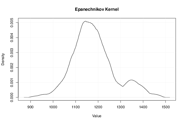
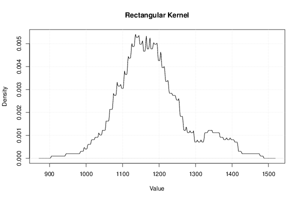
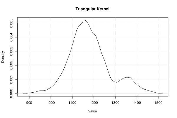
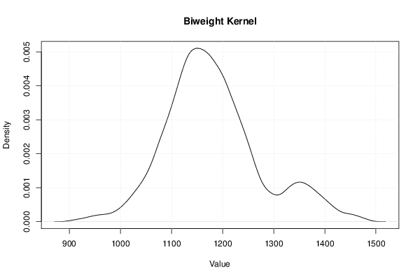
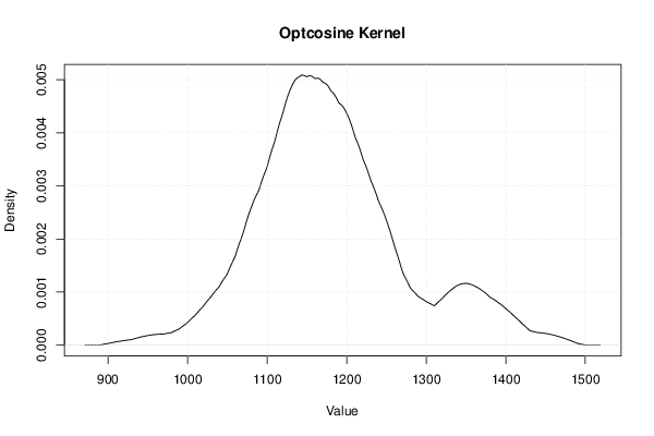
| Title produced by software | Kernel Density Estimation | ||||||||||||||||||||||||||||||||||||||||||||||||||||||||||||||||||||||||||||||||||||||
| Date of computation | Mon, 12 Aug 2013 12:02:09 -0400 | ||||||||||||||||||||||||||||||||||||||||||||||||||||||||||||||||||||||||||||||||||||||
| Cite this page as follows | Statistical Computations at FreeStatistics.org, Office for Research Development and Education, URL https://freestatistics.org/blog/index.php?v=date/2013/Aug/12/t1376323367izz0wjlc2cy1bag.htm/, Retrieved Sun, 28 Apr 2024 05:19:35 +0000 | ||||||||||||||||||||||||||||||||||||||||||||||||||||||||||||||||||||||||||||||||||||||
| Statistical Computations at FreeStatistics.org, Office for Research Development and Education, URL https://freestatistics.org/blog/index.php?pk=211051, Retrieved Sun, 28 Apr 2024 05:19:35 +0000 | |||||||||||||||||||||||||||||||||||||||||||||||||||||||||||||||||||||||||||||||||||||||
| QR Codes: | |||||||||||||||||||||||||||||||||||||||||||||||||||||||||||||||||||||||||||||||||||||||
|
| |||||||||||||||||||||||||||||||||||||||||||||||||||||||||||||||||||||||||||||||||||||||
| Original text written by user: | |||||||||||||||||||||||||||||||||||||||||||||||||||||||||||||||||||||||||||||||||||||||
| IsPrivate? | No (this computation is public) | ||||||||||||||||||||||||||||||||||||||||||||||||||||||||||||||||||||||||||||||||||||||
| User-defined keywords | Anthony Van Dyck | ||||||||||||||||||||||||||||||||||||||||||||||||||||||||||||||||||||||||||||||||||||||
| Estimated Impact | 136 | ||||||||||||||||||||||||||||||||||||||||||||||||||||||||||||||||||||||||||||||||||||||
Tree of Dependent Computations | |||||||||||||||||||||||||||||||||||||||||||||||||||||||||||||||||||||||||||||||||||||||
| Family? (F = Feedback message, R = changed R code, M = changed R Module, P = changed Parameters, D = changed Data) | |||||||||||||||||||||||||||||||||||||||||||||||||||||||||||||||||||||||||||||||||||||||
| - [Univariate Data Series] [Tijdreeks 1 - stap 2] [2013-08-12 11:07:04] [c4bfab449d963e708b9482b0c0d301bf] - P [Univariate Data Series] [Tijdreeks A - Stap 2] [2013-08-12 11:17:51] [fffbdc2eb6bf36a612a50d50ad291a0a] - RMP [Histogram] [Tijdreeks A - Stap 3] [2013-08-12 11:22:38] [fffbdc2eb6bf36a612a50d50ad291a0a] - R P [Histogram] [Tijdreeks A -stap 5] [2013-08-12 11:38:26] [c4bfab449d963e708b9482b0c0d301bf] - P [Histogram] [Tijdreeks A -stap 5] [2013-08-12 11:42:06] [c4bfab449d963e708b9482b0c0d301bf] - RMP [Harrell-Davis Quantiles] [Tijdreeks A - sta...] [2013-08-12 12:35:57] [fffbdc2eb6bf36a612a50d50ad291a0a] - R P [Harrell-Davis Quantiles] [Tijdreeks A - sta...] [2013-08-12 12:48:29] [c4bfab449d963e708b9482b0c0d301bf] - RMP [(Partial) Autocorrelation Function] [Tijdreeks A - sta...] [2013-08-12 13:54:06] [fffbdc2eb6bf36a612a50d50ad291a0a] - RM D [Kernel Density Estimation] [Tijdreeks B - stap 4] [2013-08-12 16:02:09] [c43b2753d6eee680db8e2d052715ef09] [Current] | |||||||||||||||||||||||||||||||||||||||||||||||||||||||||||||||||||||||||||||||||||||||
| Feedback Forum | |||||||||||||||||||||||||||||||||||||||||||||||||||||||||||||||||||||||||||||||||||||||
Post a new message | |||||||||||||||||||||||||||||||||||||||||||||||||||||||||||||||||||||||||||||||||||||||
Dataset | |||||||||||||||||||||||||||||||||||||||||||||||||||||||||||||||||||||||||||||||||||||||
| Dataseries X: | |||||||||||||||||||||||||||||||||||||||||||||||||||||||||||||||||||||||||||||||||||||||
1160 1220 1100 1030 1110 1160 1170 1090 1160 1210 1250 1200 1180 1210 950 1070 1120 1220 1170 1120 1180 1250 1240 1230 1120 1330 990 1110 1090 1210 1220 1220 1100 1200 1320 1180 1110 1300 1060 1130 1160 1260 1210 1190 1130 1170 1370 1170 1040 1340 1050 1130 1150 1220 1210 1150 1130 1150 1440 1160 1130 1350 1050 1150 1120 1170 1100 1120 1210 1170 1370 1170 1110 1320 1060 1150 1160 1230 1140 1100 1270 1160 1380 1150 1180 1370 1080 1160 1230 1210 1130 1110 1250 1210 1370 1080 1220 1360 1120 1150 1180 1250 1040 1180 1250 1120 1430 1150 | |||||||||||||||||||||||||||||||||||||||||||||||||||||||||||||||||||||||||||||||||||||||
Tables (Output of Computation) | |||||||||||||||||||||||||||||||||||||||||||||||||||||||||||||||||||||||||||||||||||||||
| |||||||||||||||||||||||||||||||||||||||||||||||||||||||||||||||||||||||||||||||||||||||
Figures (Output of Computation) | |||||||||||||||||||||||||||||||||||||||||||||||||||||||||||||||||||||||||||||||||||||||
Input Parameters & R Code | |||||||||||||||||||||||||||||||||||||||||||||||||||||||||||||||||||||||||||||||||||||||
| Parameters (Session): | |||||||||||||||||||||||||||||||||||||||||||||||||||||||||||||||||||||||||||||||||||||||
| par1 = 60 ; par2 = 1 ; par3 = 1 ; par4 = 0 ; par5 = 12 ; par6 = White Noise ; par7 = 0.95 ; | |||||||||||||||||||||||||||||||||||||||||||||||||||||||||||||||||||||||||||||||||||||||
| Parameters (R input): | |||||||||||||||||||||||||||||||||||||||||||||||||||||||||||||||||||||||||||||||||||||||
| par1 = 0 ; par2 = no ; par3 = 512 ; | |||||||||||||||||||||||||||||||||||||||||||||||||||||||||||||||||||||||||||||||||||||||
| R code (references can be found in the software module): | |||||||||||||||||||||||||||||||||||||||||||||||||||||||||||||||||||||||||||||||||||||||
if (par1 == '0') bw <- 'nrd0' | |||||||||||||||||||||||||||||||||||||||||||||||||||||||||||||||||||||||||||||||||||||||