Free Statistics
of Irreproducible Research!
Description of Statistical Computation | |||||||||||||||||||||||||||||||||||||||||||||||||||||||||||||||||||||||||||||||||||||
|---|---|---|---|---|---|---|---|---|---|---|---|---|---|---|---|---|---|---|---|---|---|---|---|---|---|---|---|---|---|---|---|---|---|---|---|---|---|---|---|---|---|---|---|---|---|---|---|---|---|---|---|---|---|---|---|---|---|---|---|---|---|---|---|---|---|---|---|---|---|---|---|---|---|---|---|---|---|---|---|---|---|---|---|---|---|
| Author's title | |||||||||||||||||||||||||||||||||||||||||||||||||||||||||||||||||||||||||||||||||||||
| Author | *Unverified author* | ||||||||||||||||||||||||||||||||||||||||||||||||||||||||||||||||||||||||||||||||||||
| R Software Module | rwasp_notchedbox1.wasp | ||||||||||||||||||||||||||||||||||||||||||||||||||||||||||||||||||||||||||||||||||||
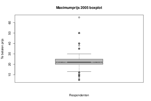
| Title produced by software | Notched Boxplots | ||||||||||||||||||||||||||||||||||||||||||||||||||||||||||||||||||||||||||||||||||||
| Date of computation | Tue, 26 Feb 2013 15:31:34 -0500 | ||||||||||||||||||||||||||||||||||||||||||||||||||||||||||||||||||||||||||||||||||||
| Cite this page as follows | Statistical Computations at FreeStatistics.org, Office for Research Development and Education, URL https://freestatistics.org/blog/index.php?v=date/2013/Feb/26/t1361910746pupjna8m6lmukd7.htm/, Retrieved Sun, 05 May 2024 04:58:03 +0000 | ||||||||||||||||||||||||||||||||||||||||||||||||||||||||||||||||||||||||||||||||||||
| Statistical Computations at FreeStatistics.org, Office for Research Development and Education, URL https://freestatistics.org/blog/index.php?pk=207108, Retrieved Sun, 05 May 2024 04:58:03 +0000 | |||||||||||||||||||||||||||||||||||||||||||||||||||||||||||||||||||||||||||||||||||||
| QR Codes: | |||||||||||||||||||||||||||||||||||||||||||||||||||||||||||||||||||||||||||||||||||||
|
| |||||||||||||||||||||||||||||||||||||||||||||||||||||||||||||||||||||||||||||||||||||
| Original text written by user: | |||||||||||||||||||||||||||||||||||||||||||||||||||||||||||||||||||||||||||||||||||||
| IsPrivate? | No (this computation is public) | ||||||||||||||||||||||||||||||||||||||||||||||||||||||||||||||||||||||||||||||||||||
| User-defined keywords | |||||||||||||||||||||||||||||||||||||||||||||||||||||||||||||||||||||||||||||||||||||
| Estimated Impact | 133 | ||||||||||||||||||||||||||||||||||||||||||||||||||||||||||||||||||||||||||||||||||||
Tree of Dependent Computations | |||||||||||||||||||||||||||||||||||||||||||||||||||||||||||||||||||||||||||||||||||||
| Family? (F = Feedback message, R = changed R code, M = changed R Module, P = changed Parameters, D = changed Data) | |||||||||||||||||||||||||||||||||||||||||||||||||||||||||||||||||||||||||||||||||||||
| - [Notched Boxplots] [] [2013-02-26 20:31:34] [8f84a338303fe8d74ac0d8ad91c8b331] [Current] - R PD [Notched Boxplots] [] [2014-08-17 22:19:23] [f974b105a61ab974a820d469d59cfaf7] - RMP [Harrell-Davis Quantiles] [] [2014-08-17 22:39:29] [f974b105a61ab974a820d469d59cfaf7] - RMP [Harrell-Davis Quantiles] [] [2014-08-17 22:47:58] [f974b105a61ab974a820d469d59cfaf7] - R D [Notched Boxplots] [] [2014-08-18 05:14:28] [f974b105a61ab974a820d469d59cfaf7] - RMPD [Harrell-Davis Quantiles] [] [2014-08-18 05:22:13] [f974b105a61ab974a820d469d59cfaf7] - R P [Harrell-Davis Quantiles] [] [2014-08-18 05:24:34] [f974b105a61ab974a820d469d59cfaf7] - RMP [Central Tendency] [] [2014-08-18 05:30:11] [f974b105a61ab974a820d469d59cfaf7] - RMP [Mean Plot] [] [2014-08-18 05:40:18] [f974b105a61ab974a820d469d59cfaf7] - RMP [(Partial) Autocorrelation Function] [] [2014-08-18 06:01:25] [f974b105a61ab974a820d469d59cfaf7] - R P [(Partial) Autocorrelation Function] [] [2014-08-18 06:09:45] [f974b105a61ab974a820d469d59cfaf7] - RMP [Standard Deviation Plot] [] [2014-08-18 06:17:47] [f974b105a61ab974a820d469d59cfaf7] - RMP [Standard Deviation-Mean Plot] [] [2014-08-18 06:30:50] [f974b105a61ab974a820d469d59cfaf7] - RMP [Classical Decomposition] [] [2014-08-18 06:45:26] [f974b105a61ab974a820d469d59cfaf7] - RMPD [Univariate Data Series] [] [2014-08-18 07:05:48] [f85cc8f00ef4b762f0a6fdfddc793773] - R [Univariate Data Series] [] [2014-08-18 07:07:33] [f85cc8f00ef4b762f0a6fdfddc793773] - RM [Histogram] [] [2014-08-18 07:10:06] [f85cc8f00ef4b762f0a6fdfddc793773] - RM [Kernel Density Estimation] [] [2014-08-18 07:12:07] [f974b105a61ab974a820d469d59cfaf7] - RM [Notched Boxplots] [] [2014-08-18 07:14:57] [f974b105a61ab974a820d469d59cfaf7] - RM [Harrell-Davis Quantiles] [] [2014-08-18 07:16:46] [f974b105a61ab974a820d469d59cfaf7] - RM [Harrell-Davis Quantiles] [] [2014-08-18 07:19:42] [f974b105a61ab974a820d469d59cfaf7] - RM [Central Tendency] [] [2014-08-18 07:24:13] [f974b105a61ab974a820d469d59cfaf7] - RM [Mean versus Median] [] [2014-08-18 07:29:41] [f974b105a61ab974a820d469d59cfaf7] - RM [Mean Plot] [] [2014-08-18 07:32:51] [f974b105a61ab974a820d469d59cfaf7] - RM [(Partial) Autocorrelation Function] [] [2014-08-18 07:41:46] [f974b105a61ab974a820d469d59cfaf7] - R [(Partial) Autocorrelation Function] [] [2014-08-18 07:52:14] [f974b105a61ab974a820d469d59cfaf7] - RM [Variability] [] [2014-08-18 07:54:08] [f974b105a61ab974a820d469d59cfaf7] - RM [Standard Deviation-Mean Plot] [] [2014-08-18 07:59:48] [f974b105a61ab974a820d469d59cfaf7] - RM [Classical Decomposition] [] [2014-08-18 08:06:30] [f974b105a61ab974a820d469d59cfaf7] - RM [Exponential Smoothing] [] [2014-08-18 08:23:15] [f974b105a61ab974a820d469d59cfaf7] | |||||||||||||||||||||||||||||||||||||||||||||||||||||||||||||||||||||||||||||||||||||
| Feedback Forum | |||||||||||||||||||||||||||||||||||||||||||||||||||||||||||||||||||||||||||||||||||||
Post a new message | |||||||||||||||||||||||||||||||||||||||||||||||||||||||||||||||||||||||||||||||||||||
Dataset | |||||||||||||||||||||||||||||||||||||||||||||||||||||||||||||||||||||||||||||||||||||
| Dataseries X: | |||||||||||||||||||||||||||||||||||||||||||||||||||||||||||||||||||||||||||||||||||||
20 25 15 15 25 25 25 21 30 25 20 40 13 30 25 20 25 20 25 20 20 15 15 12 20 5 20 15 25 22 20 22 25 20 20 35 30 25 20 20 20 25 25 15 20 35 25 25 30 23 10 22 25 25 22 30 20 25 25 22 25 25 25 22 25 12 18 20 20 22 30 25 22 20 50 30 25 20 30 22 25 30 22 25 22 22 25 25 25 20 22 15 20 30 20 25 30 35 22 12 30 15 10 30 9 25 20 20 35 25 35 30 12 25 15 25 25 20 20 6 15 40 20 40 25 25 20 15 15 22 24 22 20 25 25 25 35 40 20 22 22 20 25 25 18 25 20 25 30 20 22 35 22 25 25 25 25 22 23 35 15 25 18 22 25 25 28 30 20 25 25 30 22 30 10 10 25 20 22 25 25 15 22 25 25 28 22 30 25 20 25 25 20 30 20 30 50 19 20 28 20 25 35 25 25 15 16 20 20 25 30 20 25 25 25 20 20 25 25 30 22 20 25 25 18 18 20 25 25 30 25 20 25 20 20 20 22 18 22 20 15 25 25 20 25 15 22 25 25 15 12 25 30 22 15 22 25 12 18 30 25 25 40 24 25 15 25 20 25 25 25 20 30 20 25 30 22 25 25 25 50 19 50 25 35 20 20 20 20 20 25 25 25 20 20 20 20 25 18 25 22 22 30 30 8 20 25 30 50 22 20 10 25 25 25 25 18 25 20 25 30 18 20 25 22 22 20 20 25 20 20 20 20 25 20 10 20 25 30 25 50 30 30 50 15 25 25 22 20 22 30 25 18 22 22 30 40 25 20 10 20 9 15 20 15 20 30 12 15 12 20 15 12 25 20 25 25 25 30 20 25 15 15 22 10 15 10 20 25 20 20 38 20 20 20 40 25 25 30 25 10 20 25 12 15 25 20 22 22 20 25 25 25 15 40 20 20 16 25 15 20 25 20 30 50 20 25 20 30 30 25 25 12 25 25 25 20 20 20 15 20 25 15 25 50 30 20 20 25 12 15 20 20 35 22 15 18 30 22 12 12 20 20 15 25 15 20 20 25 18 30 20 25 25 25 20 20 25 20 22 15 15 22 20 10 25 20 20 15 12 20 5 20 15 15 25 25 25 15 25 22 25 20 18 22 25 35 25 25 25 35 30 22 30 50 15 25 24 20 25 25 25 12 15 22 25 25 25 25 15 20 20 15 35 30 20 22 65 20 25 22 20 25 25 20 25 15 20 12 15 10 25 15 30 35 25 25 25 25 25 40 40 25 25 20 25 25 22 25 30 25 25 30 25 25 30 25 25 20 22 22 20 25 22 25 22 40 25 25 25 22 20 35 20 35 25 22 25 25 25 25 25 40 25 30 25 20 25 25 30 22 22 20 15 15 25 25 20 20 15 25 15 20 22 25 15 15 18 5 15 25 18 40 25 25 20 30 20 25 25 25 22 22 25 25 30 25 25 25 25 20 20 25 25 25 25 20 30 25 22 30 20 20 30 25 25 30 20 25 25 24 25 30 18 15 22 22 25 22 22 25 15 20 22 18 35 20 20 20 25 25 30 15 25 22 26 25 20 25 25 25 22 25 25 20 22 30 15 30 25 20 25 25 35 22 20 25 20 20 18 20 22 25 10 20 25 20 20 30 25 20 15 20 25 10 20 25 22 22 25 25 15 25 20 10 25 16 25 35 25 15 25 25 30 25 10 22 20 25 20 20 25 22 18 30 19 25 20 25 20 25 20 22 12 30 12 22 25 25 25 25 30 30 10 22 22 25 20 22 20 25 20 15 25 20 25 20 30 15 40 25 20 22 22 30 20 40 20 25 20 25 20 50 50 25 25 40 30 22 30 20 25 25 30 25 25 20 18 18 28 25 22 15 40 40 12 12 18 12 25 26 18 25 22 15 25 15 15 15 25 15 12 22 20 20 25 20 12 9 15 12 15 25 20 20 15 15 30 21 25 22 22 50 15 25 15 25 22 18 50 20 50 20 20 30 25 20 22 25 50 40 25 25 25 25 30 40 25 30 20 | |||||||||||||||||||||||||||||||||||||||||||||||||||||||||||||||||||||||||||||||||||||
Tables (Output of Computation) | |||||||||||||||||||||||||||||||||||||||||||||||||||||||||||||||||||||||||||||||||||||
| |||||||||||||||||||||||||||||||||||||||||||||||||||||||||||||||||||||||||||||||||||||
Figures (Output of Computation) | |||||||||||||||||||||||||||||||||||||||||||||||||||||||||||||||||||||||||||||||||||||
Input Parameters & R Code | |||||||||||||||||||||||||||||||||||||||||||||||||||||||||||||||||||||||||||||||||||||
| Parameters (Session): | |||||||||||||||||||||||||||||||||||||||||||||||||||||||||||||||||||||||||||||||||||||
| par1 = grey ; | |||||||||||||||||||||||||||||||||||||||||||||||||||||||||||||||||||||||||||||||||||||
| Parameters (R input): | |||||||||||||||||||||||||||||||||||||||||||||||||||||||||||||||||||||||||||||||||||||
| par1 = grey ; | |||||||||||||||||||||||||||||||||||||||||||||||||||||||||||||||||||||||||||||||||||||
| R code (references can be found in the software module): | |||||||||||||||||||||||||||||||||||||||||||||||||||||||||||||||||||||||||||||||||||||
par1 <- 'grey' | |||||||||||||||||||||||||||||||||||||||||||||||||||||||||||||||||||||||||||||||||||||