Free Statistics
of Irreproducible Research!
Description of Statistical Computation | |||||||||||||||||||||||||||||||||||||||||||||||||||||||||||||||||||||||||||||||||||||||||||||||||||||||||
|---|---|---|---|---|---|---|---|---|---|---|---|---|---|---|---|---|---|---|---|---|---|---|---|---|---|---|---|---|---|---|---|---|---|---|---|---|---|---|---|---|---|---|---|---|---|---|---|---|---|---|---|---|---|---|---|---|---|---|---|---|---|---|---|---|---|---|---|---|---|---|---|---|---|---|---|---|---|---|---|---|---|---|---|---|---|---|---|---|---|---|---|---|---|---|---|---|---|---|---|---|---|---|---|---|---|
| Author's title | |||||||||||||||||||||||||||||||||||||||||||||||||||||||||||||||||||||||||||||||||||||||||||||||||||||||||
| Author | *Unverified author* | ||||||||||||||||||||||||||||||||||||||||||||||||||||||||||||||||||||||||||||||||||||||||||||||||||||||||
| R Software Module | rwasp_bootstrapplot1.wasp | ||||||||||||||||||||||||||||||||||||||||||||||||||||||||||||||||||||||||||||||||||||||||||||||||||||||||
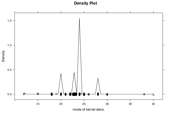
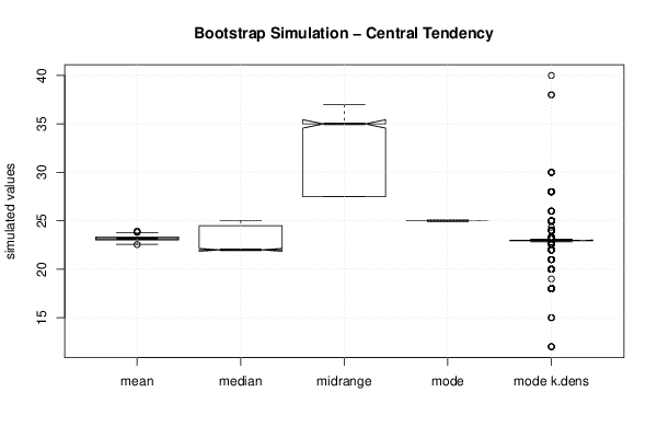
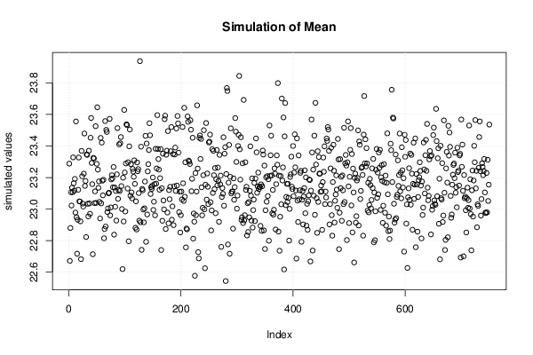
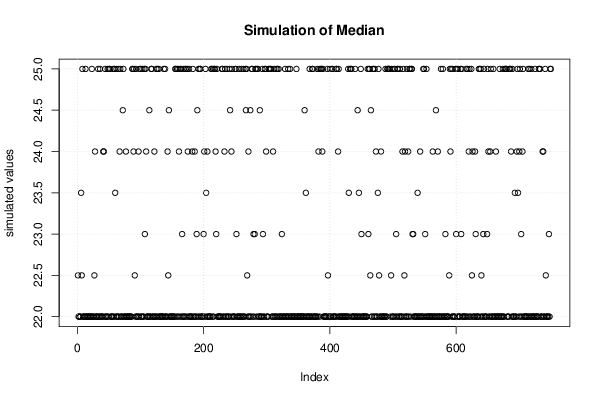
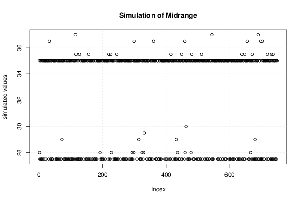
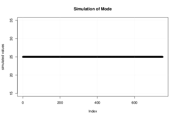
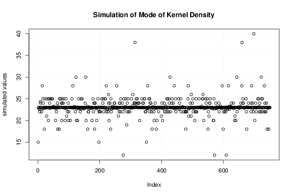
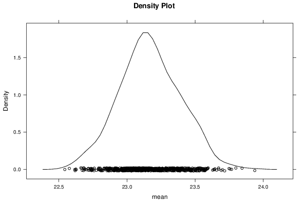
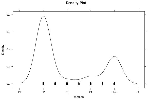
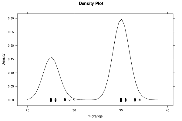
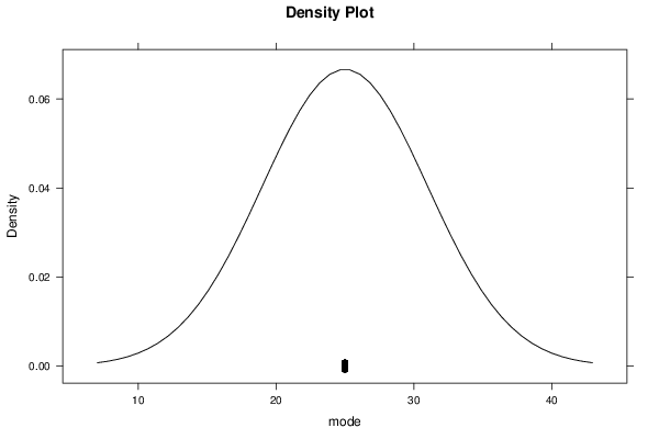
| Title produced by software | Bootstrap Plot - Central Tendency | ||||||||||||||||||||||||||||||||||||||||||||||||||||||||||||||||||||||||||||||||||||||||||||||||||||||||
| Date of computation | Wed, 09 Jan 2013 06:45:46 -0500 | ||||||||||||||||||||||||||||||||||||||||||||||||||||||||||||||||||||||||||||||||||||||||||||||||||||||||
| Cite this page as follows | Statistical Computations at FreeStatistics.org, Office for Research Development and Education, URL https://freestatistics.org/blog/index.php?v=date/2013/Jan/09/t1357732017ji8e74xkgjy9lf3.htm/, Retrieved Mon, 29 Apr 2024 10:09:03 +0000 | ||||||||||||||||||||||||||||||||||||||||||||||||||||||||||||||||||||||||||||||||||||||||||||||||||||||||
| Statistical Computations at FreeStatistics.org, Office for Research Development and Education, URL https://freestatistics.org/blog/index.php?pk=205105, Retrieved Mon, 29 Apr 2024 10:09:03 +0000 | |||||||||||||||||||||||||||||||||||||||||||||||||||||||||||||||||||||||||||||||||||||||||||||||||||||||||
| QR Codes: | |||||||||||||||||||||||||||||||||||||||||||||||||||||||||||||||||||||||||||||||||||||||||||||||||||||||||
|
| |||||||||||||||||||||||||||||||||||||||||||||||||||||||||||||||||||||||||||||||||||||||||||||||||||||||||
| Original text written by user: | |||||||||||||||||||||||||||||||||||||||||||||||||||||||||||||||||||||||||||||||||||||||||||||||||||||||||
| IsPrivate? | No (this computation is public) | ||||||||||||||||||||||||||||||||||||||||||||||||||||||||||||||||||||||||||||||||||||||||||||||||||||||||
| User-defined keywords | |||||||||||||||||||||||||||||||||||||||||||||||||||||||||||||||||||||||||||||||||||||||||||||||||||||||||
| Estimated Impact | 158 | ||||||||||||||||||||||||||||||||||||||||||||||||||||||||||||||||||||||||||||||||||||||||||||||||||||||||
Tree of Dependent Computations | |||||||||||||||||||||||||||||||||||||||||||||||||||||||||||||||||||||||||||||||||||||||||||||||||||||||||
| Family? (F = Feedback message, R = changed R code, M = changed R Module, P = changed Parameters, D = changed Data) | |||||||||||||||||||||||||||||||||||||||||||||||||||||||||||||||||||||||||||||||||||||||||||||||||||||||||
| - [Bootstrap Plot - Central Tendency] [maximumprijzen st...] [2013-01-09 11:37:25] [251e6916fe5b161c77205c1c19032f50] - R P [Bootstrap Plot - Central Tendency] [maximumprijzen st...] [2013-01-09 11:42:15] [251e6916fe5b161c77205c1c19032f50] - P [Bootstrap Plot - Central Tendency] [maximumprijzen st...] [2013-01-09 11:45:46] [3e2b14d12dd0cca2f2b67dfbdf2cdaf9] [Current] - RMPD [Blocked Bootstrap Plot - Central Tendency] [niet werkende wer...] [2013-01-09 16:05:30] [251e6916fe5b161c77205c1c19032f50] - R P [Blocked Bootstrap Plot - Central Tendency] [niet werkende wer...] [2013-01-09 16:11:50] [251e6916fe5b161c77205c1c19032f50] - R P [Blocked Bootstrap Plot - Central Tendency] [niet werkende wer...] [2013-01-09 16:14:18] [251e6916fe5b161c77205c1c19032f50] - RMPD [Variability] [maximumprijzen st...] [2013-01-09 16:49:45] [251e6916fe5b161c77205c1c19032f50] - RMPD [Standard Deviation Plot] [aantal nieuwe ins...] [2013-01-09 16:55:24] [251e6916fe5b161c77205c1c19032f50] - RMPD [Standard Deviation-Mean Plot] [aantal inschrijvi...] [2013-01-09 17:03:14] [251e6916fe5b161c77205c1c19032f50] - RMP [Variability] [aantal niet werke...] [2013-01-09 17:09:53] [251e6916fe5b161c77205c1c19032f50] - RMP [Variability] [niet werkende wer...] [2013-01-09 17:09:53] [251e6916fe5b161c77205c1c19032f50] - RMP [Standard Deviation Plot] [niet werkende wer...] [2013-01-09 17:15:26] [251e6916fe5b161c77205c1c19032f50] - RMP [Standard Deviation-Mean Plot] [niet werkende wer...] [2013-01-09 17:29:23] [251e6916fe5b161c77205c1c19032f50] - RMPD [Classical Decomposition] [aantal nieuwe ins...] [2013-01-09 17:44:28] [251e6916fe5b161c77205c1c19032f50] - RMP [Classical Decomposition] [niet werkende wer...] [2013-01-09 18:03:13] [251e6916fe5b161c77205c1c19032f50] - RMPD [Exponential Smoothing] [aantal nieuwe ins...] [2013-01-09 18:12:47] [2f0f353a58a70fd7baf0f5141860d820] - RMP [Exponential Smoothing] [niet werkende wer...] [2013-01-09 18:14:43] [2f0f353a58a70fd7baf0f5141860d820] | |||||||||||||||||||||||||||||||||||||||||||||||||||||||||||||||||||||||||||||||||||||||||||||||||||||||||
| Feedback Forum | |||||||||||||||||||||||||||||||||||||||||||||||||||||||||||||||||||||||||||||||||||||||||||||||||||||||||
Post a new message | |||||||||||||||||||||||||||||||||||||||||||||||||||||||||||||||||||||||||||||||||||||||||||||||||||||||||
Dataset | |||||||||||||||||||||||||||||||||||||||||||||||||||||||||||||||||||||||||||||||||||||||||||||||||||||||||
| Dataseries X: | |||||||||||||||||||||||||||||||||||||||||||||||||||||||||||||||||||||||||||||||||||||||||||||||||||||||||
20 25 15 15 25 25 25 21 30 25 20 40 13 30 25 20 25 20 25 20 20 15 15 12 20 5 20 15 25 22 20 22 25 20 20 35 30 25 20 20 20 25 25 15 20 35 25 25 30 23 10 22 25 25 22 30 20 25 25 22 25 25 25 22 25 12 18 20 20 22 30 25 22 20 50 30 25 20 30 22 25 30 22 25 22 22 25 25 25 20 22 15 20 30 20 25 30 35 22 12 30 15 10 30 9 25 20 20 35 25 35 30 12 25 15 25 25 20 20 6 15 40 20 40 25 25 20 15 15 22 24 22 20 25 25 25 35 40 20 22 22 20 25 25 18 25 20 25 30 20 22 35 22 25 25 25 25 22 23 35 15 25 18 22 25 25 28 30 20 25 25 30 22 30 10 10 25 20 22 25 25 15 22 25 25 28 22 30 25 20 25 25 20 30 20 30 50 19 20 28 20 25 35 25 25 15 16 20 20 25 30 20 25 25 25 20 20 25 25 30 22 20 25 25 18 18 20 25 25 30 25 20 25 20 20 20 22 18 22 20 15 25 25 20 25 15 22 25 25 15 12 25 30 22 15 22 25 12 18 30 25 25 40 24 25 15 25 20 25 25 25 20 30 20 25 30 22 25 25 25 50 19 50 25 35 20 20 20 20 20 25 25 25 20 20 20 20 25 18 25 22 22 30 30 8 20 25 30 50 22 20 10 25 25 25 25 18 25 20 25 30 18 20 25 22 22 20 20 25 20 20 20 20 25 20 10 20 25 30 25 50 30 30 50 15 25 25 22 20 22 30 25 18 22 22 30 40 25 20 10 20 9 15 20 15 20 30 12 15 12 20 15 12 25 20 25 25 25 30 20 25 15 15 22 10 15 10 20 25 20 20 38 20 20 20 40 25 25 30 25 10 20 25 12 15 25 20 22 22 20 25 25 25 15 40 20 20 16 25 15 20 25 20 30 50 20 25 20 30 30 25 25 12 25 25 25 20 20 20 15 20 25 15 25 50 30 20 20 25 12 15 20 20 35 22 15 18 30 22 12 12 20 20 15 25 15 20 20 25 18 30 20 25 25 25 20 20 25 20 22 15 15 22 20 10 25 20 20 15 12 20 5 20 15 15 25 25 25 15 25 22 25 20 18 22 25 35 25 25 25 35 30 22 30 50 15 25 24 20 25 25 25 12 15 22 25 25 25 25 15 20 20 15 35 30 20 22 65 20 25 22 20 25 25 20 25 15 20 12 15 10 25 15 30 35 25 25 25 25 25 40 40 25 25 20 25 25 22 25 30 25 25 30 25 25 30 25 25 20 22 22 20 25 22 25 22 40 25 25 25 22 20 35 20 35 25 22 25 25 25 25 25 40 25 30 25 20 25 25 30 22 22 20 15 15 25 25 20 20 15 25 15 20 22 25 15 15 18 5 15 25 18 40 25 25 20 30 20 25 25 25 22 22 25 25 30 25 25 25 25 20 20 25 25 25 25 20 30 25 22 30 20 20 30 25 25 30 20 25 25 24 25 30 18 15 22 22 25 22 22 25 15 20 22 18 35 20 20 20 25 25 30 15 25 22 26 25 20 25 25 25 22 25 25 20 22 30 15 30 25 20 25 25 35 22 20 25 20 20 18 20 22 25 10 20 25 20 20 30 25 20 15 20 25 10 20 25 22 22 25 25 15 25 20 10 25 16 25 35 25 15 25 25 30 25 10 22 20 25 20 20 25 22 18 30 19 25 20 25 20 25 20 22 12 30 12 22 25 25 25 25 30 30 10 22 22 25 20 22 20 25 20 15 25 20 25 20 30 15 40 25 20 22 22 30 20 40 20 25 20 25 20 50 50 25 25 40 30 22 30 20 25 25 30 25 25 20 18 18 28 25 22 15 40 40 12 12 18 12 25 26 18 25 22 15 25 15 15 15 25 15 12 22 20 20 25 20 12 9 15 12 15 25 20 20 15 15 30 21 25 22 22 50 15 25 15 25 22 18 50 20 50 20 20 30 25 20 22 25 50 40 25 25 25 25 30 40 25 30 20 | |||||||||||||||||||||||||||||||||||||||||||||||||||||||||||||||||||||||||||||||||||||||||||||||||||||||||
Tables (Output of Computation) | |||||||||||||||||||||||||||||||||||||||||||||||||||||||||||||||||||||||||||||||||||||||||||||||||||||||||
| |||||||||||||||||||||||||||||||||||||||||||||||||||||||||||||||||||||||||||||||||||||||||||||||||||||||||
Figures (Output of Computation) | |||||||||||||||||||||||||||||||||||||||||||||||||||||||||||||||||||||||||||||||||||||||||||||||||||||||||
Input Parameters & R Code | |||||||||||||||||||||||||||||||||||||||||||||||||||||||||||||||||||||||||||||||||||||||||||||||||||||||||
| Parameters (Session): | |||||||||||||||||||||||||||||||||||||||||||||||||||||||||||||||||||||||||||||||||||||||||||||||||||||||||
| par1 = 750 ; par2 = 5 ; par3 = 0 ; | |||||||||||||||||||||||||||||||||||||||||||||||||||||||||||||||||||||||||||||||||||||||||||||||||||||||||
| Parameters (R input): | |||||||||||||||||||||||||||||||||||||||||||||||||||||||||||||||||||||||||||||||||||||||||||||||||||||||||
| par1 = 750 ; par2 = 5 ; par3 = 0 ; | |||||||||||||||||||||||||||||||||||||||||||||||||||||||||||||||||||||||||||||||||||||||||||||||||||||||||
| R code (references can be found in the software module): | |||||||||||||||||||||||||||||||||||||||||||||||||||||||||||||||||||||||||||||||||||||||||||||||||||||||||
par1 <- as.numeric(par1) | |||||||||||||||||||||||||||||||||||||||||||||||||||||||||||||||||||||||||||||||||||||||||||||||||||||||||