Free Statistics
of Irreproducible Research!
Description of Statistical Computation | |||||||||||||||||||||
|---|---|---|---|---|---|---|---|---|---|---|---|---|---|---|---|---|---|---|---|---|---|
| Author's title | |||||||||||||||||||||
| Author | *Unverified author* | ||||||||||||||||||||
| R Software Module | rwasp_meanplot.wasp | ||||||||||||||||||||
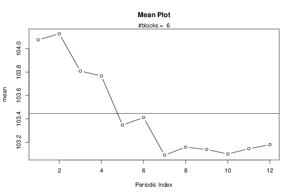
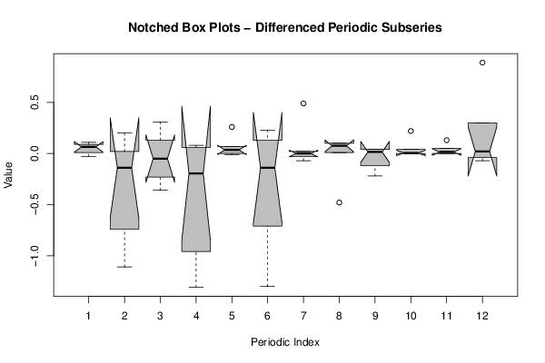
| Title produced by software | Mean Plot | ||||||||||||||||||||
| Date of computation | Thu, 07 Mar 2013 06:03:59 -0500 | ||||||||||||||||||||
| Cite this page as follows | Statistical Computations at FreeStatistics.org, Office for Research Development and Education, URL https://freestatistics.org/blog/index.php?v=date/2013/Mar/07/t13626543113sb5a15a1jmcry7.htm/, Retrieved Tue, 30 Apr 2024 14:16:45 +0000 | ||||||||||||||||||||
| Statistical Computations at FreeStatistics.org, Office for Research Development and Education, URL https://freestatistics.org/blog/index.php?pk=207591, Retrieved Tue, 30 Apr 2024 14:16:45 +0000 | |||||||||||||||||||||
| QR Codes: | |||||||||||||||||||||
|
| |||||||||||||||||||||
| Original text written by user: | Mean plot: gem farma consumptieprijzen | ||||||||||||||||||||
| IsPrivate? | No (this computation is public) | ||||||||||||||||||||
| User-defined keywords | Mean plot: gem farma consumptieprijzen | ||||||||||||||||||||
| Estimated Impact | 65 | ||||||||||||||||||||
Tree of Dependent Computations | |||||||||||||||||||||
| Family? (F = Feedback message, R = changed R code, M = changed R Module, P = changed Parameters, D = changed Data) | |||||||||||||||||||||
| - [Mean Plot] [] [2013-03-07 11:03:59] [0941a6a4eb2aa1312aa94e558e86fae5] [Current] | |||||||||||||||||||||
| Feedback Forum | |||||||||||||||||||||
Post a new message | |||||||||||||||||||||
Dataset | |||||||||||||||||||||
| Dataseries X: | |||||||||||||||||||||
105,71 105,82 105,82 105,72 105,76 105,80 105,09 105,06 105,16 105,20 105,21 105,23 105,19 105,16 104,88 104,52 104,09 104,35 104,48 104,47 104,55 104,59 104,59 104,72 104,65 104,72 104,92 105,05 103,74 103,81 103,79 104,28 103,80 103,80 104,02 104,02 104,91 104,97 103,86 104,17 103,21 103,21 101,91 101,84 101,91 101,79 101,79 101,79 102,09 102,18 102,20 101,97 102,05 102,04 101,78 101,79 101,80 101,83 101,83 101,88 101,90 101,91 101,17 101,17 101,23 101,26 101,49 101,51 101,61 101,39 101,43 101,44 | |||||||||||||||||||||
Tables (Output of Computation) | |||||||||||||||||||||
| |||||||||||||||||||||
Figures (Output of Computation) | |||||||||||||||||||||
Input Parameters & R Code | |||||||||||||||||||||
| Parameters (Session): | |||||||||||||||||||||
| par1 = 12 ; | |||||||||||||||||||||
| Parameters (R input): | |||||||||||||||||||||
| par1 = 12 ; | |||||||||||||||||||||
| R code (references can be found in the software module): | |||||||||||||||||||||
par1 <- as.numeric(par1) | |||||||||||||||||||||