Repository of Reproducible Computations

Free Statistics

of Irreproducible Research!

Author's title

Author

*Unverified author*

R Software Module

rwasp_histogram.wasp

Title produced by software

Histogram

Date of computation

Thu, 07 Mar 2013 10:52:30 -0500

Cite this page as follows

Statistical Computations at FreeStatistics.org, Office for Research Development and Education, URL https://freestatistics.org/blog/index.php?v=date/2013/Mar/07/t1362671580aktpoac5sxejyv0.htm/, Retrieved Tue, 30 Apr 2024 11:09:31 +0000

Statistical Computations at FreeStatistics.org, Office for Research Development and Education, URL https://freestatistics.org/blog/index.php?pk=207608, Retrieved Tue, 30 Apr 2024 11:09:31 +0000

QR Codes:

Paste this QR Code to cite your computation.

Original text written by user:

IsPrivate?

No (this computation is public)

User-defined keywords

Estimated Impact

118

Family? (F = Feedback message, R = changed R code, M = changed R Module, P = changed Parameters, D = changed Data)

-     [Histogram] [tu berlin lina1 k...] [2012-07-11 21:49:14] [74be16979710d4c4e7c6647856088456]
- R PD  [Histogram] [Ana1MathSS12 Klau...] [2012-07-17 14:33:20] [74be16979710d4c4e7c6647856088456]
- R PD      [Histogram] [Klausurergebnisse...] [2013-03-07 15:52:30] [d41d8cd98f00b204e9800998ecf8427e] [Current]

Feedback Forum

Post a new message

Dataseries X:

Download CSV

Histogram

Boxplots

51.5
58.5
51.0
75.5
68.0
73.0
53.0
39.0
32.5
47.5
51.0
71.0
44.0
54.5
89.0
70.0
46.5
45.5
66.0
48.0
47.0
54.5
56.5
46.0
33.5
43.5
44.0
59.5
87.5
60.5
78.5
75.0
44.5
81.5
53.5
48.0
53.5
60.5
37.0
47.0
67.5
51.5
36.0
28.0
56.0
23.5
67.0
70.0
43.5
46.0
48.5
40.5
35.0
62.5
36.5
67.5
45.5
57.5
75.5
78.0
19.0
57.0
84.0
78.0
90.0
75.5
80.5
28.0
54.0
46.0
63.0
51.5
48.0
69.0
39.0
91.5
59.5
65.5
70.5
83.5
74.0
46.5
55.0
68.5
48.5
76.0
41.5
73.5
60.5
63.5
70.5
84.5
63.5
51.0
84.0
48.5
88.5
79.0
70.5
72.0
58.5
62.0
48.5
31.5

Summary of computational transaction
Raw Input	view raw input (R code)
Raw Output	view raw output of R engine
Computing time	1 seconds
R Server	'Herman Ole Andreas Wold' @ wold.wessa.net

\begin{tabular}{lllllllll}
\hline
Summary of computational transaction \tabularnewline
Raw Input & view raw input (R code)  \tabularnewline
Raw Output & view raw output of R engine  \tabularnewline
Computing time & 1 seconds \tabularnewline
R Server & 'Herman Ole Andreas Wold' @ wold.wessa.net \tabularnewline
\hline
\end{tabular}
%Source: https://freestatistics.org/blog/index.php?pk=207608&T=0

[TABLE]
[ROW][C]Summary of computational transaction[/C][/ROW]
[ROW][C]Raw Input[/C][C]view raw input (R code) [/C][/ROW]
[ROW][C]Raw Output[/C][C]view raw output of R engine [/C][/ROW]
[ROW][C]Computing time[/C][C]1 seconds[/C][/ROW]
[ROW][C]R Server[/C][C]'Herman Ole Andreas Wold' @ wold.wessa.net[/C][/ROW]
[/TABLE]
Source: https://freestatistics.org/blog/index.php?pk=207608&T=0

Globally Unique Identifier (entire table): ba.freestatistics.org/blog/index.php?pk=207608&T=0

As an alternative you can also use a QR Code:

The GUIDs for individual cells are displayed in the table below:

Summary of computational transaction
Raw Input	view raw input (R code)
Raw Output	view raw output of R engine
Computing time	1 seconds
R Server	'Herman Ole Andreas Wold' @ wold.wessa.net

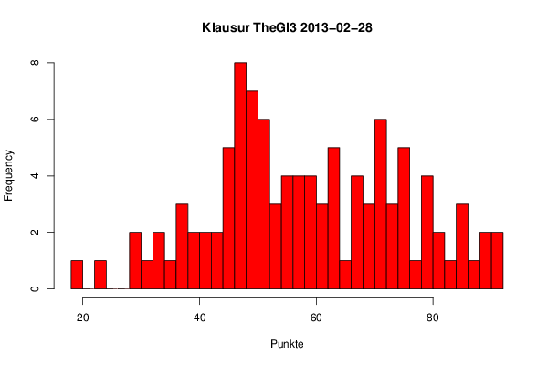
Frequency Table (Histogram)
Bins	Midpoint	Abs. Frequency	Rel. Frequency	Cumul. Rel. Freq.	Density
[18,20[	19	1	0.009615	0.009615	0.004808
[20,22[	21	0	0	0.009615	0
[22,24[	23	1	0.009615	0.019231	0.004808
[24,26[	25	0	0	0.019231	0
[26,28[	27	0	0	0.019231	0
[28,30[	29	2	0.019231	0.038462	0.009615
[30,32[	31	1	0.009615	0.048077	0.004808
[32,34[	33	2	0.019231	0.067308	0.009615
[34,36[	35	1	0.009615	0.076923	0.004808
[36,38[	37	3	0.028846	0.105769	0.014423
[38,40[	39	2	0.019231	0.125	0.009615
[40,42[	41	2	0.019231	0.144231	0.009615
[42,44[	43	2	0.019231	0.163462	0.009615
[44,46[	45	5	0.048077	0.211538	0.024038
[46,48[	47	8	0.076923	0.288462	0.038462
[48,50[	49	7	0.067308	0.355769	0.033654
[50,52[	51	6	0.057692	0.413462	0.028846
[52,54[	53	3	0.028846	0.442308	0.014423
[54,56[	55	4	0.038462	0.480769	0.019231
[56,58[	57	4	0.038462	0.519231	0.019231
[58,60[	59	4	0.038462	0.557692	0.019231
[60,62[	61	3	0.028846	0.586538	0.014423
[62,64[	63	5	0.048077	0.634615	0.024038
[64,66[	65	1	0.009615	0.644231	0.004808
[66,68[	67	4	0.038462	0.682692	0.019231
[68,70[	69	3	0.028846	0.711538	0.014423
[70,72[	71	6	0.057692	0.769231	0.028846
[72,74[	73	3	0.028846	0.798077	0.014423
[74,76[	75	5	0.048077	0.846154	0.024038
[76,78[	77	1	0.009615	0.855769	0.004808
[78,80[	79	4	0.038462	0.894231	0.019231
[80,82[	81	2	0.019231	0.913462	0.009615
[82,84[	83	1	0.009615	0.923077	0.004808
[84,86[	85	3	0.028846	0.951923	0.014423
[86,88[	87	1	0.009615	0.961538	0.004808
[88,90[	89	2	0.019231	0.980769	0.009615
[90,92]	91	2	0.019231	1	0.009615

\begin{tabular}{lllllllll}
\hline
Frequency Table (Histogram) \tabularnewline
Bins & Midpoint & Abs. Frequency & Rel. Frequency & Cumul. Rel. Freq. & Density \tabularnewline
[18,20[ & 19 & 1 & 0.009615 & 0.009615 & 0.004808 \tabularnewline
[20,22[ & 21 & 0 & 0 & 0.009615 & 0 \tabularnewline
[22,24[ & 23 & 1 & 0.009615 & 0.019231 & 0.004808 \tabularnewline
[24,26[ & 25 & 0 & 0 & 0.019231 & 0 \tabularnewline
[26,28[ & 27 & 0 & 0 & 0.019231 & 0 \tabularnewline
[28,30[ & 29 & 2 & 0.019231 & 0.038462 & 0.009615 \tabularnewline
[30,32[ & 31 & 1 & 0.009615 & 0.048077 & 0.004808 \tabularnewline
[32,34[ & 33 & 2 & 0.019231 & 0.067308 & 0.009615 \tabularnewline
[34,36[ & 35 & 1 & 0.009615 & 0.076923 & 0.004808 \tabularnewline
[36,38[ & 37 & 3 & 0.028846 & 0.105769 & 0.014423 \tabularnewline
[38,40[ & 39 & 2 & 0.019231 & 0.125 & 0.009615 \tabularnewline
[40,42[ & 41 & 2 & 0.019231 & 0.144231 & 0.009615 \tabularnewline
[42,44[ & 43 & 2 & 0.019231 & 0.163462 & 0.009615 \tabularnewline
[44,46[ & 45 & 5 & 0.048077 & 0.211538 & 0.024038 \tabularnewline
[46,48[ & 47 & 8 & 0.076923 & 0.288462 & 0.038462 \tabularnewline
[48,50[ & 49 & 7 & 0.067308 & 0.355769 & 0.033654 \tabularnewline
[50,52[ & 51 & 6 & 0.057692 & 0.413462 & 0.028846 \tabularnewline
[52,54[ & 53 & 3 & 0.028846 & 0.442308 & 0.014423 \tabularnewline
[54,56[ & 55 & 4 & 0.038462 & 0.480769 & 0.019231 \tabularnewline
[56,58[ & 57 & 4 & 0.038462 & 0.519231 & 0.019231 \tabularnewline
[58,60[ & 59 & 4 & 0.038462 & 0.557692 & 0.019231 \tabularnewline
[60,62[ & 61 & 3 & 0.028846 & 0.586538 & 0.014423 \tabularnewline
[62,64[ & 63 & 5 & 0.048077 & 0.634615 & 0.024038 \tabularnewline
[64,66[ & 65 & 1 & 0.009615 & 0.644231 & 0.004808 \tabularnewline
[66,68[ & 67 & 4 & 0.038462 & 0.682692 & 0.019231 \tabularnewline
[68,70[ & 69 & 3 & 0.028846 & 0.711538 & 0.014423 \tabularnewline
[70,72[ & 71 & 6 & 0.057692 & 0.769231 & 0.028846 \tabularnewline
[72,74[ & 73 & 3 & 0.028846 & 0.798077 & 0.014423 \tabularnewline
[74,76[ & 75 & 5 & 0.048077 & 0.846154 & 0.024038 \tabularnewline
[76,78[ & 77 & 1 & 0.009615 & 0.855769 & 0.004808 \tabularnewline
[78,80[ & 79 & 4 & 0.038462 & 0.894231 & 0.019231 \tabularnewline
[80,82[ & 81 & 2 & 0.019231 & 0.913462 & 0.009615 \tabularnewline
[82,84[ & 83 & 1 & 0.009615 & 0.923077 & 0.004808 \tabularnewline
[84,86[ & 85 & 3 & 0.028846 & 0.951923 & 0.014423 \tabularnewline
[86,88[ & 87 & 1 & 0.009615 & 0.961538 & 0.004808 \tabularnewline
[88,90[ & 89 & 2 & 0.019231 & 0.980769 & 0.009615 \tabularnewline
[90,92] & 91 & 2 & 0.019231 & 1 & 0.009615 \tabularnewline
\hline
\end{tabular}
%Source: https://freestatistics.org/blog/index.php?pk=207608&T=1

[TABLE]
[ROW][C]Frequency Table (Histogram)[/C][/ROW]
[ROW][C]Bins[/C][C]Midpoint[/C][C]Abs. Frequency[/C][C]Rel. Frequency[/C][C]Cumul. Rel. Freq.[/C][C]Density[/C][/ROW]
[ROW][C][18,20[[/C][C]19[/C][C]1[/C][C]0.009615[/C][C]0.009615[/C][C]0.004808[/C][/ROW]
[ROW][C][20,22[[/C][C]21[/C][C]0[/C][C]0[/C][C]0.009615[/C][C]0[/C][/ROW]
[ROW][C][22,24[[/C][C]23[/C][C]1[/C][C]0.009615[/C][C]0.019231[/C][C]0.004808[/C][/ROW]
[ROW][C][24,26[[/C][C]25[/C][C]0[/C][C]0[/C][C]0.019231[/C][C]0[/C][/ROW]
[ROW][C][26,28[[/C][C]27[/C][C]0[/C][C]0[/C][C]0.019231[/C][C]0[/C][/ROW]
[ROW][C][28,30[[/C][C]29[/C][C]2[/C][C]0.019231[/C][C]0.038462[/C][C]0.009615[/C][/ROW]
[ROW][C][30,32[[/C][C]31[/C][C]1[/C][C]0.009615[/C][C]0.048077[/C][C]0.004808[/C][/ROW]
[ROW][C][32,34[[/C][C]33[/C][C]2[/C][C]0.019231[/C][C]0.067308[/C][C]0.009615[/C][/ROW]
[ROW][C][34,36[[/C][C]35[/C][C]1[/C][C]0.009615[/C][C]0.076923[/C][C]0.004808[/C][/ROW]
[ROW][C][36,38[[/C][C]37[/C][C]3[/C][C]0.028846[/C][C]0.105769[/C][C]0.014423[/C][/ROW]
[ROW][C][38,40[[/C][C]39[/C][C]2[/C][C]0.019231[/C][C]0.125[/C][C]0.009615[/C][/ROW]
[ROW][C][40,42[[/C][C]41[/C][C]2[/C][C]0.019231[/C][C]0.144231[/C][C]0.009615[/C][/ROW]
[ROW][C][42,44[[/C][C]43[/C][C]2[/C][C]0.019231[/C][C]0.163462[/C][C]0.009615[/C][/ROW]
[ROW][C][44,46[[/C][C]45[/C][C]5[/C][C]0.048077[/C][C]0.211538[/C][C]0.024038[/C][/ROW]
[ROW][C][46,48[[/C][C]47[/C][C]8[/C][C]0.076923[/C][C]0.288462[/C][C]0.038462[/C][/ROW]
[ROW][C][48,50[[/C][C]49[/C][C]7[/C][C]0.067308[/C][C]0.355769[/C][C]0.033654[/C][/ROW]
[ROW][C][50,52[[/C][C]51[/C][C]6[/C][C]0.057692[/C][C]0.413462[/C][C]0.028846[/C][/ROW]
[ROW][C][52,54[[/C][C]53[/C][C]3[/C][C]0.028846[/C][C]0.442308[/C][C]0.014423[/C][/ROW]
[ROW][C][54,56[[/C][C]55[/C][C]4[/C][C]0.038462[/C][C]0.480769[/C][C]0.019231[/C][/ROW]
[ROW][C][56,58[[/C][C]57[/C][C]4[/C][C]0.038462[/C][C]0.519231[/C][C]0.019231[/C][/ROW]
[ROW][C][58,60[[/C][C]59[/C][C]4[/C][C]0.038462[/C][C]0.557692[/C][C]0.019231[/C][/ROW]
[ROW][C][60,62[[/C][C]61[/C][C]3[/C][C]0.028846[/C][C]0.586538[/C][C]0.014423[/C][/ROW]
[ROW][C][62,64[[/C][C]63[/C][C]5[/C][C]0.048077[/C][C]0.634615[/C][C]0.024038[/C][/ROW]
[ROW][C][64,66[[/C][C]65[/C][C]1[/C][C]0.009615[/C][C]0.644231[/C][C]0.004808[/C][/ROW]
[ROW][C][66,68[[/C][C]67[/C][C]4[/C][C]0.038462[/C][C]0.682692[/C][C]0.019231[/C][/ROW]
[ROW][C][68,70[[/C][C]69[/C][C]3[/C][C]0.028846[/C][C]0.711538[/C][C]0.014423[/C][/ROW]
[ROW][C][70,72[[/C][C]71[/C][C]6[/C][C]0.057692[/C][C]0.769231[/C][C]0.028846[/C][/ROW]
[ROW][C][72,74[[/C][C]73[/C][C]3[/C][C]0.028846[/C][C]0.798077[/C][C]0.014423[/C][/ROW]
[ROW][C][74,76[[/C][C]75[/C][C]5[/C][C]0.048077[/C][C]0.846154[/C][C]0.024038[/C][/ROW]
[ROW][C][76,78[[/C][C]77[/C][C]1[/C][C]0.009615[/C][C]0.855769[/C][C]0.004808[/C][/ROW]
[ROW][C][78,80[[/C][C]79[/C][C]4[/C][C]0.038462[/C][C]0.894231[/C][C]0.019231[/C][/ROW]
[ROW][C][80,82[[/C][C]81[/C][C]2[/C][C]0.019231[/C][C]0.913462[/C][C]0.009615[/C][/ROW]
[ROW][C][82,84[[/C][C]83[/C][C]1[/C][C]0.009615[/C][C]0.923077[/C][C]0.004808[/C][/ROW]
[ROW][C][84,86[[/C][C]85[/C][C]3[/C][C]0.028846[/C][C]0.951923[/C][C]0.014423[/C][/ROW]
[ROW][C][86,88[[/C][C]87[/C][C]1[/C][C]0.009615[/C][C]0.961538[/C][C]0.004808[/C][/ROW]
[ROW][C][88,90[[/C][C]89[/C][C]2[/C][C]0.019231[/C][C]0.980769[/C][C]0.009615[/C][/ROW]
[ROW][C][90,92][/C][C]91[/C][C]2[/C][C]0.019231[/C][C]1[/C][C]0.009615[/C][/ROW]
[/TABLE]
Source: https://freestatistics.org/blog/index.php?pk=207608&T=1

Globally Unique Identifier (entire table): ba.freestatistics.org/blog/index.php?pk=207608&T=1

As an alternative you can also use a QR Code:

The GUIDs for individual cells are displayed in the table below:

Frequency Table (Histogram)
Bins	Midpoint	Abs. Frequency	Rel. Frequency	Cumul. Rel. Freq.	Density
[18,20[	19	1	0.009615	0.009615	0.004808
[20,22[	21	0	0	0.009615	0
[22,24[	23	1	0.009615	0.019231	0.004808
[24,26[	25	0	0	0.019231	0
[26,28[	27	0	0	0.019231	0
[28,30[	29	2	0.019231	0.038462	0.009615
[30,32[	31	1	0.009615	0.048077	0.004808
[32,34[	33	2	0.019231	0.067308	0.009615
[34,36[	35	1	0.009615	0.076923	0.004808
[36,38[	37	3	0.028846	0.105769	0.014423
[38,40[	39	2	0.019231	0.125	0.009615
[40,42[	41	2	0.019231	0.144231	0.009615
[42,44[	43	2	0.019231	0.163462	0.009615
[44,46[	45	5	0.048077	0.211538	0.024038
[46,48[	47	8	0.076923	0.288462	0.038462
[48,50[	49	7	0.067308	0.355769	0.033654
[50,52[	51	6	0.057692	0.413462	0.028846
[52,54[	53	3	0.028846	0.442308	0.014423
[54,56[	55	4	0.038462	0.480769	0.019231
[56,58[	57	4	0.038462	0.519231	0.019231
[58,60[	59	4	0.038462	0.557692	0.019231
[60,62[	61	3	0.028846	0.586538	0.014423
[62,64[	63	5	0.048077	0.634615	0.024038
[64,66[	65	1	0.009615	0.644231	0.004808
[66,68[	67	4	0.038462	0.682692	0.019231
[68,70[	69	3	0.028846	0.711538	0.014423
[70,72[	71	6	0.057692	0.769231	0.028846
[72,74[	73	3	0.028846	0.798077	0.014423
[74,76[	75	5	0.048077	0.846154	0.024038
[76,78[	77	1	0.009615	0.855769	0.004808
[78,80[	79	4	0.038462	0.894231	0.019231
[80,82[	81	2	0.019231	0.913462	0.009615
[82,84[	83	1	0.009615	0.923077	0.004808
[84,86[	85	3	0.028846	0.951923	0.014423
[86,88[	87	1	0.009615	0.961538	0.004808
[88,90[	89	2	0.019231	0.980769	0.009615
[90,92]	91	2	0.019231	1	0.009615

Figure 1

PNG link

Postscript link

PDF link

Parameters (Session):

par1 = 15 ; par2 = red ; par3 = TRUE ; par4 = Unknown ;

Parameters (R input):

par1 = 90 ; par2 = red ; par3 = FALSE ; par4 = Unknown ;

R code (references can be found in the software module):

par1 <- as.numeric(par1)
if (par3 == 'TRUE') par3 <- TRUE
if (par3 == 'FALSE') par3 <- FALSE
if (par4 == 'Unknown') par1 <- as.numeric(par1)
if (par4 == 'Interval/Ratio') par1 <- as.numeric(par1)
if (par4 == '3-point Likert') par1 <- c(1:3 - 0.5, 3.5)
if (par4 == '4-point Likert') par1 <- c(1:4 - 0.5, 4.5)
if (par4 == '5-point Likert') par1 <- c(1:5 - 0.5, 5.5)
if (par4 == '6-point Likert') par1 <- c(1:6 - 0.5, 6.5)
if (par4 == '7-point Likert') par1 <- c(1:7 - 0.5, 7.5)
if (par4 == '8-point Likert') par1 <- c(1:8 - 0.5, 8.5)
if (par4 == '9-point Likert') par1 <- c(1:9 - 0.5, 9.5)
if (par4 == '10-point Likert') par1 <- c(1:10 - 0.5, 10.5)
bitmap(file='test1.png')
if(is.numeric(x[1])) {
if (is.na(par1)) {
myhist<-hist(x,col=par2,main=main,xlab=xlab,right=par3)
} else {
if (par1 < 0) par1 <- 3
if (par1 > 50) par1 <- 50
myhist<-hist(x,breaks=par1,col=par2,main=main,xlab=xlab,right=par3)
}
} else {
plot(mytab <- table(x),col=par2,main='Frequency Plot',xlab=xlab,ylab='Absolute Frequency')
}
dev.off()
if(is.numeric(x[1])) {
myhist
n <- length(x)
load(file='createtable')
a<-table.start()
a<-table.row.start(a)
a<-table.element(a,hyperlink('histogram.htm','Frequency Table (Histogram)',''),6,TRUE)
a<-table.row.end(a)
a<-table.row.start(a)
a<-table.element(a,'Bins',header=TRUE)
a<-table.element(a,'Midpoint',header=TRUE)
a<-table.element(a,'Abs. Frequency',header=TRUE)
a<-table.element(a,'Rel. Frequency',header=TRUE)
a<-table.element(a,'Cumul. Rel. Freq.',header=TRUE)
a<-table.element(a,'Density',header=TRUE)
a<-table.row.end(a)
crf <- 0
if (par3 == FALSE) mybracket <- '[' else mybracket <- ']'
mynumrows <- (length(myhist$breaks)-1)
for (i in 1:mynumrows) {
a<-table.row.start(a)
if (i == 1)
dum <- paste('[',myhist$breaks[i],sep='')
else
dum <- paste(mybracket,myhist$breaks[i],sep='')
dum <- paste(dum,myhist$breaks[i+1],sep=',')
if (i==mynumrows)
dum <- paste(dum,']',sep='')
else
dum <- paste(dum,mybracket,sep='')
a<-table.element(a,dum,header=TRUE)
a<-table.element(a,myhist$mids[i])
a<-table.element(a,myhist$counts[i])
rf <- myhist$counts[i]/n
crf <- crf + rf
a<-table.element(a,round(rf,6))
a<-table.element(a,round(crf,6))
a<-table.element(a,round(myhist$density[i],6))
a<-table.row.end(a)
}
a<-table.end(a)
table.save(a,file='mytable.tab')
} else {
mytab
reltab <- mytab / sum(mytab)
n <- length(mytab)
load(file='createtable')
a<-table.start()
a<-table.row.start(a)
a<-table.element(a,'Frequency Table (Categorical Data)',3,TRUE)
a<-table.row.end(a)
a<-table.row.start(a)
a<-table.element(a,'Category',header=TRUE)
a<-table.element(a,'Abs. Frequency',header=TRUE)
a<-table.element(a,'Rel. Frequency',header=TRUE)
a<-table.row.end(a)
for (i in 1:n) {
a<-table.row.start(a)
a<-table.element(a,labels(mytab)$x[i],header=TRUE)
a<-table.element(a,mytab[i])
a<-table.element(a,round(reltab[i],4))
a<-table.row.end(a)
}
a<-table.end(a)
table.save(a,file='mytable1.tab')
}

Free Statistics

Description of Statistical Computation

Tree of Dependent Computations

Dataset

Tables (Output of Computation)

Figures (Output of Computation)

Input Parameters & R Code