Free Statistics
of Irreproducible Research!
Description of Statistical Computation | |||||||||||||||||||||
|---|---|---|---|---|---|---|---|---|---|---|---|---|---|---|---|---|---|---|---|---|---|
| Author's title | |||||||||||||||||||||
| Author | *Unverified author* | ||||||||||||||||||||
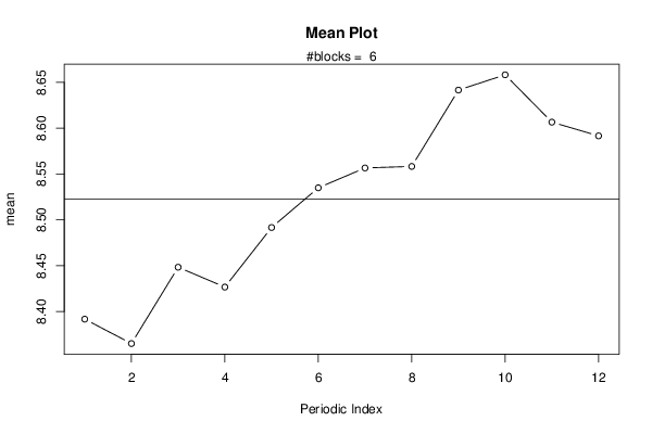
| R Software Module | rwasp_meanplot.wasp | ||||||||||||||||||||
| Title produced by software | Mean Plot | ||||||||||||||||||||
| Date of computation | Thu, 07 Mar 2013 11:15:35 -0500 | ||||||||||||||||||||
| Cite this page as follows | Statistical Computations at FreeStatistics.org, Office for Research Development and Education, URL https://freestatistics.org/blog/index.php?v=date/2013/Mar/07/t136267303945an8cezwb2y0nl.htm/, Retrieved Tue, 30 Apr 2024 17:30:28 +0000 | ||||||||||||||||||||
| Statistical Computations at FreeStatistics.org, Office for Research Development and Education, URL https://freestatistics.org/blog/index.php?pk=207652, Retrieved Tue, 30 Apr 2024 17:30:28 +0000 | |||||||||||||||||||||
| QR Codes: | |||||||||||||||||||||
|
| |||||||||||||||||||||
| Original text written by user: | |||||||||||||||||||||
| IsPrivate? | No (this computation is public) | ||||||||||||||||||||
| User-defined keywords | |||||||||||||||||||||
| Estimated Impact | 56 | ||||||||||||||||||||
Tree of Dependent Computations | |||||||||||||||||||||
| Family? (F = Feedback message, R = changed R code, M = changed R Module, P = changed Parameters, D = changed Data) | |||||||||||||||||||||
| - [Mean Plot] [] [2013-03-07 16:15:35] [138d0669d5f70cc84d77479d15dc4661] [Current] | |||||||||||||||||||||
| Feedback Forum | |||||||||||||||||||||
Post a new message | |||||||||||||||||||||
Dataset | |||||||||||||||||||||
| Dataseries X: | |||||||||||||||||||||
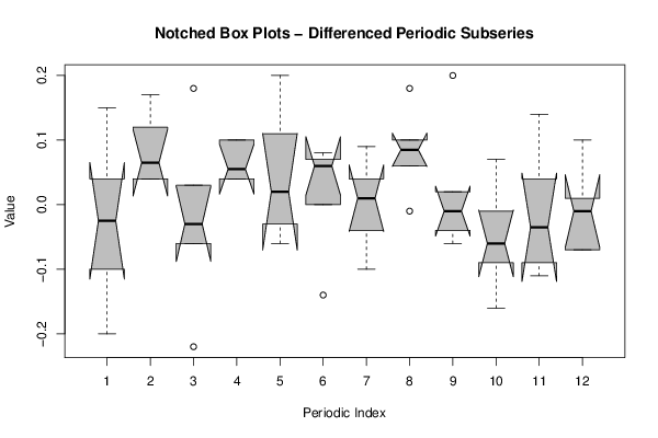
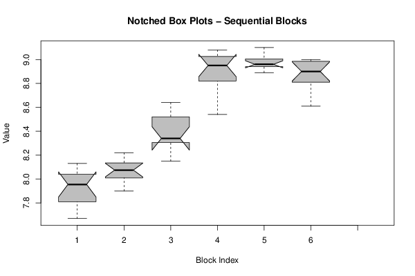
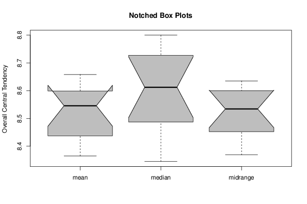
7,72 7,67 7,84 7,79 7,83 7,94 8,02 8,06 8,12 8,13 7,97 8,01 8 7,9 7,99 8,02 8,08 8,02 8,07 8,11 8,19 8,16 8,08 8,22 8,15 8,19 8,31 8,3 8,34 8,31 8,38 8,34 8,44 8,64 8,6 8,61 8,54 8,69 8,73 8,91 9,01 9,08 8,94 9,03 9,02 8,96 9,03 8,94 8,95 8,95 8,99 8,93 8,98 8,95 9,02 8,92 9,1 9,06 8,97 8,89 8,99 8,79 8,83 8,61 8,71 8,91 8,91 8,89 8,98 9 8,99 8,88 | |||||||||||||||||||||
Tables (Output of Computation) | |||||||||||||||||||||
| |||||||||||||||||||||
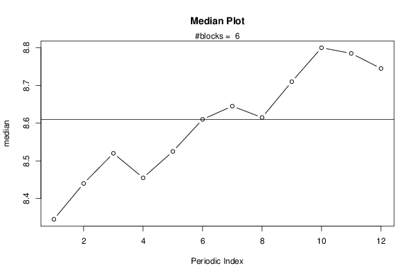
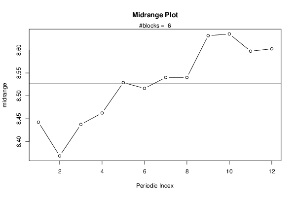
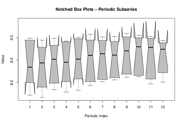
Figures (Output of Computation) | |||||||||||||||||||||
Input Parameters & R Code | |||||||||||||||||||||
| Parameters (Session): | |||||||||||||||||||||
| par1 = 12 ; | |||||||||||||||||||||
| Parameters (R input): | |||||||||||||||||||||
| par1 = 12 ; | |||||||||||||||||||||
| R code (references can be found in the software module): | |||||||||||||||||||||
par1 <- as.numeric(par1) | |||||||||||||||||||||