Free Statistics
of Irreproducible Research!
Description of Statistical Computation | |||||||||||||||||||||
|---|---|---|---|---|---|---|---|---|---|---|---|---|---|---|---|---|---|---|---|---|---|
| Author's title | |||||||||||||||||||||
| Author | *Unverified author* | ||||||||||||||||||||
| R Software Module | rwasp_meanplot.wasp | ||||||||||||||||||||
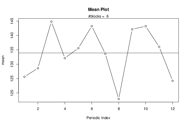
| Title produced by software | Mean Plot | ||||||||||||||||||||
| Date of computation | Sat, 09 Mar 2013 09:16:07 -0500 | ||||||||||||||||||||
| Cite this page as follows | Statistical Computations at FreeStatistics.org, Office for Research Development and Education, URL https://freestatistics.org/blog/index.php?v=date/2013/Mar/09/t1362838619wvjc2t0vdhg7esj.htm/, Retrieved Sat, 27 Apr 2024 14:07:27 +0000 | ||||||||||||||||||||
| Statistical Computations at FreeStatistics.org, Office for Research Development and Education, URL https://freestatistics.org/blog/index.php?pk=207680, Retrieved Sat, 27 Apr 2024 14:07:27 +0000 | |||||||||||||||||||||
| QR Codes: | |||||||||||||||||||||
|
| |||||||||||||||||||||
| Original text written by user: | |||||||||||||||||||||
| IsPrivate? | No (this computation is public) | ||||||||||||||||||||
| User-defined keywords | |||||||||||||||||||||
| Estimated Impact | 171 | ||||||||||||||||||||
Tree of Dependent Computations | |||||||||||||||||||||
| Family? (F = Feedback message, R = changed R code, M = changed R Module, P = changed Parameters, D = changed Data) | |||||||||||||||||||||
| - [Mean Plot] [Buitenlandse hand...] [2013-03-09 14:16:07] [aebd7ed62a520371cf0fbdf4b97f0dea] [Current] | |||||||||||||||||||||
| Feedback Forum | |||||||||||||||||||||
Post a new message | |||||||||||||||||||||
Dataset | |||||||||||||||||||||
| Dataseries X: | |||||||||||||||||||||
122,27 124,69 147,56 120,03 136,01 138,16 122,87 112,22 137,35 139,08 139,64 121,12 132,37 130,69 149,41 130,72 139,14 146,55 137,35 122,73 138,97 154,73 143,4 123,88 140,25 142,39 143,81 153,58 144,71 153,84 151,3 121,92 153,05 149,29 118,81 109,19 103,68 106,94 114,43 107,87 103,14 117,02 112,44 95,85 123,86 121,83 121,95 120,34 113,32 117,31 141,69 130,35 127,28 148,1 131,21 120,37 146,91 144,04 141,77 132,15 142,04 149,77 172,31 150,24 163,23 155,92 146,96 134,51 152,83 150,54 150,98 138,82 | |||||||||||||||||||||
Tables (Output of Computation) | |||||||||||||||||||||
| |||||||||||||||||||||
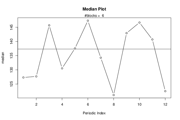
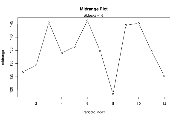
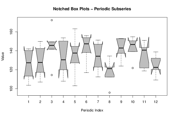
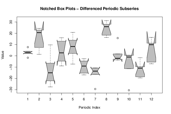
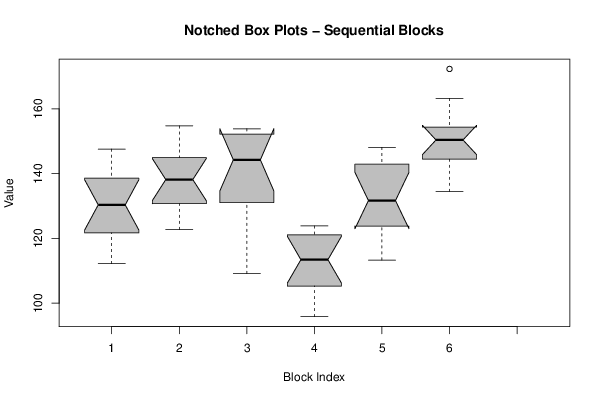
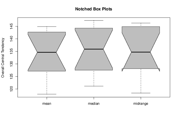
Figures (Output of Computation) | |||||||||||||||||||||
Input Parameters & R Code | |||||||||||||||||||||
| Parameters (Session): | |||||||||||||||||||||
| par1 = 12 ; | |||||||||||||||||||||
| Parameters (R input): | |||||||||||||||||||||
| par1 = 12 ; | |||||||||||||||||||||
| R code (references can be found in the software module): | |||||||||||||||||||||
par1 <- as.numeric(par1) | |||||||||||||||||||||