Free Statistics

of Irreproducible Research!

Author's title

Author*The author of this computation has been verified*
R Software Modulerwasp_CARE Data Boxplot.wasp
Title produced by softwareCARE Data - Boxplots and Scatterplot Matrix
Date of computationWed, 22 May 2013 10:16:57 -0400
Cite this page as followsStatistical Computations at FreeStatistics.org, Office for Research Development and Education, URL https://freestatistics.org/blog/index.php?v=date/2013/May/22/t1369232236sztmxq3lzk4vx5k.htm/, Retrieved Sat, 27 Apr 2024 19:04:39 +0000
Statistical Computations at FreeStatistics.org, Office for Research Development and Education, URL https://freestatistics.org/blog/index.php?pk=209718, Retrieved Sat, 27 Apr 2024 19:04:39 +0000
QR Codes:

Original text written by user:
IsPrivate?No (this computation is public)
User-defined keywords
Estimated Impact92
Family? (F = Feedback message, R = changed R code, M = changed R Module, P = changed Parameters, D = changed Data)
-     [Simple Linear Regression] [RAD BPVT Regression] [2013-05-18 11:35:15] [98fd0e87c3eb04e0cc2efde01dbafab6]
- RMPD    [CARE Data - Boxplots and Scatterplot Matrix] [boxplots] [2013-05-22 14:16:57] [ab0de2774b73a706e6b03b0c8de36087] [Current]
Feedback Forum

Post a new message
Dataseries X:
29	-6.5
21	-7.33
50	49.33
23	-11
35	-2.67
36	-8.33
32	9
44	9.67
42	2.33
39	-12.3
20	-6
73	5.67
38	28.33
43	12
50	-2
32	-11.3
24	1.33
24	3
59	-4.67
41	-5
24	-13
44	2.33
66	37.67
40	7.5
24	5
31	-5.67
45	-4
60	30
35	15.33
39	2


Summary of computational transaction
Raw Inputview raw input (R code)
Raw Outputview raw output of R engine
Computing time3 seconds
R Server'Sir Maurice George Kendall' @ kendall.wessa.net

\begin{tabular}{lllllllll}
\hline
Summary of computational transaction \tabularnewline
Raw Input & view raw input (R code)  \tabularnewline
Raw Output & view raw output of R engine  \tabularnewline
Computing time & 3 seconds \tabularnewline
R Server & 'Sir Maurice George Kendall' @ kendall.wessa.net \tabularnewline
\hline
\end{tabular}
%Source: https://freestatistics.org/blog/index.php?pk=209718&T=0

[TABLE]
[ROW][C]Summary of computational transaction[/C][/ROW]
[ROW][C]Raw Input[/C][C]view raw input (R code) [/C][/ROW]
[ROW][C]Raw Output[/C][C]view raw output of R engine [/C][/ROW]
[ROW][C]Computing time[/C][C]3 seconds[/C][/ROW]
[ROW][C]R Server[/C][C]'Sir Maurice George Kendall' @ kendall.wessa.net[/C][/ROW]
[/TABLE]
Source: https://freestatistics.org/blog/index.php?pk=209718&T=0

Globally Unique Identifier (entire table): ba.freestatistics.org/blog/index.php?pk=209718&T=0

As an alternative you can also use a QR Code:  

The GUIDs for individual cells are displayed in the table below:

Summary of computational transaction
Raw Inputview raw input (R code)
Raw Outputview raw output of R engine
Computing time3 seconds
R Server'Sir Maurice George Kendall' @ kendall.wessa.net


\begin{tabular}{lllllllll}
\hline
Boxplot statistics \tabularnewline
Variable & lower whisker & lower hinge & median & upper hinge & upper whisker \tabularnewline
BV & 20 & 29 & 38.5 & 44 & 66 \tabularnewline
RAD & -13 & -6 & 1.665 & 9 & 30 \tabularnewline
\hline
\end{tabular}
%Source: https://freestatistics.org/blog/index.php?pk=209718&T=1

[TABLE]
[ROW][C]Boxplot statistics[/C][/ROW]
[ROW][C]Variable[/C][C]lower whisker[/C][C]lower hinge[/C][C]median[/C][C]upper hinge[/C][C]upper whisker[/C][/ROW]
[ROW][C]BV[/C][C]20[/C][C]29[/C][C]38.5[/C][C]44[/C][C]66[/C][/ROW]
[ROW][C]RAD[/C][C]-13[/C][C]-6[/C][C]1.665[/C][C]9[/C][C]30[/C][/ROW]
[/TABLE]
Source: https://freestatistics.org/blog/index.php?pk=209718&T=1

Globally Unique Identifier (entire table): ba.freestatistics.org/blog/index.php?pk=209718&T=1

As an alternative you can also use a QR Code:  

The GUIDs for individual cells are displayed in the table below:

Boxplot statistics
Variablelower whiskerlower hingemedianupper hingeupper whisker
BV202938.54466
RAD-13-61.665930


Boxplot Notches
Variablelower boundmedianupper bound
BV34.1738.542.83
RAD-2.6621.6655.992

\begin{tabular}{lllllllll}
\hline
Boxplot Notches \tabularnewline
Variable & lower bound & median & upper bound \tabularnewline
BV & 34.17 & 38.5 & 42.83 \tabularnewline
RAD & -2.662 & 1.665 & 5.992 \tabularnewline
\hline
\end{tabular}
%Source: https://freestatistics.org/blog/index.php?pk=209718&T=2

[TABLE]
[ROW][C]Boxplot Notches[/C][/ROW]
[ROW][C]Variable[/C][C]lower bound[/C][C]median[/C][C]upper bound[/C][/ROW]
[ROW][C]BV[/C][C]34.17[/C][C]38.5[/C][C]42.83[/C][/ROW]
[ROW][C]RAD[/C][C]-2.662[/C][C]1.665[/C][C]5.992[/C][/ROW]
[/TABLE]
Source: https://freestatistics.org/blog/index.php?pk=209718&T=2

Globally Unique Identifier (entire table): ba.freestatistics.org/blog/index.php?pk=209718&T=2

As an alternative you can also use a QR Code:  

The GUIDs for individual cells are displayed in the table below:

Boxplot Notches
Variablelower boundmedianupper bound
BV34.1738.542.83
RAD-2.6621.6655.992


Boxplot Means
Variabletrimmed meanunbiased SD
BV38.7713.43
RAD4.02415.13

\begin{tabular}{lllllllll}
\hline
Boxplot Means \tabularnewline
Variable & trimmed mean & unbiased SD \tabularnewline
BV & 38.77 & 13.43 \tabularnewline
RAD & 4.024 & 15.13 \tabularnewline
\hline
\end{tabular}
%Source: https://freestatistics.org/blog/index.php?pk=209718&T=3

[TABLE]
[ROW][C]Boxplot Means[/C][/ROW]
[ROW][C]Variable[/C][C]trimmed mean[/C][C]unbiased SD[/C][/ROW]
[ROW][C]BV[/C][C]38.77[/C][C]13.43[/C][/ROW]
[ROW][C]RAD[/C][C]4.024[/C][C]15.13[/C][/ROW]
[/TABLE]
Source: https://freestatistics.org/blog/index.php?pk=209718&T=3

Globally Unique Identifier (entire table): ba.freestatistics.org/blog/index.php?pk=209718&T=3

As an alternative you can also use a QR Code:  

The GUIDs for individual cells are displayed in the table below:

Boxplot Means
Variabletrimmed meanunbiased SD
BV38.7713.43
RAD4.02415.13


Parameters (Session):
par1 = 3 ; par2 = TRUE ; par3 = 0 ;
Parameters (R input):
par1 = 3 ; par2 = TRUE ; par3 = 0 ;
R code (references can be found in the software module):
par1 <- as.numeric(par1) #colour
par2<- as.logical(par2) # Notches ?
par3<-as.numeric(par3) # % trim
if(par3>45){par3<-45;warning('trim limited to 45%')}
if(par3<0){par3<-0;warning('negative trim makes no sense. Trim is zero.')}
lotrm<-as.integer(length(y[1,])*par3/100)+1
hitrm<-as.integer(length(y[1,])*(100-par3)/100)
y1<-array(dim=c(dim(y)[1], hitrm-lotrm+1), dimnames=list(dimnames(y)[[1]], 1:(hitrm-lotrm+1) ))
for(i in 1:dim(y)[1]){
tmp<-order(y[i,])
y1[i,]<- y[i, tmp[lotrm:hitrm] ]
}
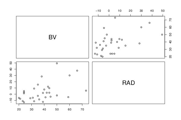
bitmap(file='test2.png')
pairs(t(y))
dev.off()
y<-y1
z <- as.data.frame(t(y))
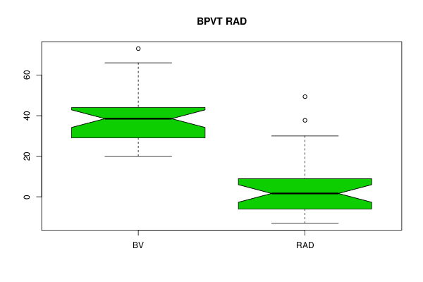
bitmap(file='test1.png')
(r<-boxplot(z ,xlab=xlab,ylab=ylab,main=main,notch=par2,col=par1))
dev.off()
load(file='createtable')
a<-table.start()
a<-table.row.start(a)
a<-table.element(a,hyperlink('overview.htm','Boxplot statistics','Boxplot overview'),6,TRUE)
a<-table.row.end(a)
a<-table.row.start(a)
a<-table.element(a,'Variable',1,TRUE)
a<-table.element(a,hyperlink('lower_whisker.htm','lower whisker','definition of lower whisker'),1,TRUE)
a<-table.element(a,hyperlink('lower_hinge.htm','lower hinge','definition of lower hinge'),1,TRUE)
a<-table.element(a,hyperlink('central_tendency.htm','median','definitions about measures of central tendency'),1,TRUE)
a<-table.element(a,hyperlink('upper_hinge.htm','upper hinge','definition of upper hinge'),1,TRUE)
a<-table.element(a,hyperlink('upper_whisker.htm','upper whisker','definition of upper whisker'),1,TRUE)
a<-table.row.end(a)
for (i in 1:length(y[,1]))
{
a<-table.row.start(a)
a<-table.element(a,dimnames(t(x))[[2]][i],1,TRUE)
for (j in 1:5)
{
a<-table.element(a,signif(r$stats[j,i], digits=4))
}
a<-table.row.end(a)
}
a<-table.end(a)
table.save(a,file='mytable.tab')
if (par2){
a<-table.start()
a<-table.row.start(a)
a<-table.element(a,'Boxplot Notches',4,TRUE)
a<-table.row.end(a)
a<-table.row.start(a)
a<-table.element(a,'Variable',1,TRUE)
a<-table.element(a,'lower bound',1,TRUE)
a<-table.element(a,'median',1,TRUE)
a<-table.element(a,'upper bound',1,TRUE)
a<-table.row.end(a)
for (i in 1:length(y[,1]))
{
a<-table.row.start(a)
a<-table.element(a,dimnames(t(x))[[2]][i],1,TRUE)
a<-table.element(a,signif(r$conf[1,i], digits=4))
a<-table.element(a, signif(r$stats[3,i], digits=4))
a<-table.element(a,signif(r$conf[2,i], digits=4))
a<-table.row.end(a)
}
a<-table.end(a)
table.save(a,file='mytable1.tab')
}
a<-table.start()
a<-table.row.start(a)
a<-table.element(a,'Boxplot Means',4,TRUE)
a<-table.row.end(a)
a<-table.row.start(a)
a<-table.element(a,'Variable',1,TRUE)
a<-table.element(a,hyperlink('trimmed_mean.htm','trimmed mean','definition of trimmed mean'),1,TRUE)
a<-table.element(a,hyperlink('unbiased1.htm','unbiased SD','definition of unbiased SD'),1,TRUE)
a<-table.row.end(a)
for (i in 1:length(y[,1]))
{
a<-table.row.start(a)
a<-table.element(a,dimnames(t(x))[[2]][i],1,TRUE)
a<-table.element(a,signif(mean(z[i], trim=par3/100, na.rm=TRUE), digits=4))
a<-table.element(a,signif(sd(z[i], na.rm=TRUE), digits=4))
a<-table.row.end(a)
}
a<-table.end(a)
table.save(a,file='mytable2.tab')