Free Statistics

of Irreproducible Research!

Author's title

Author*The author of this computation has been verified*
R Software Modulerwasp_structuraltimeseries.wasp
Title produced by softwareStructural Time Series Models
Date of computationThu, 14 Nov 2013 07:19:34 -0500
Cite this page as followsStatistical Computations at FreeStatistics.org, Office for Research Development and Education, URL https://freestatistics.org/blog/index.php?v=date/2013/Nov/14/t13844315856o0gbrqbf69uj6n.htm/, Retrieved Mon, 29 Apr 2024 10:04:21 +0000
Statistical Computations at FreeStatistics.org, Office for Research Development and Education, URL https://freestatistics.org/blog/index.php?pk=225298, Retrieved Mon, 29 Apr 2024 10:04:21 +0000
QR Codes:

Original text written by user:
IsPrivate?No (this computation is public)
User-defined keywords
Estimated Impact61
Family? (F = Feedback message, R = changed R code, M = changed R Module, P = changed Parameters, D = changed Data)
-       [Structural Time Series Models] [dlkslyqvg] [2013-11-14 12:19:34] [e931f330ae8eb739e69629b6955c783c] [Current]
Feedback Forum

Post a new message
Dataseries X:
1045620
1050293
1030185
1015746
999514
990204
962206
947314
958768


Summary of computational transaction
Raw Inputview raw input (R code)
Raw Outputview raw output of R engine
Computing time4 seconds
R Server'Sir Ronald Aylmer Fisher' @ fisher.wessa.net

\begin{tabular}{lllllllll}
\hline
Summary of computational transaction \tabularnewline
Raw Input & view raw input (R code)  \tabularnewline
Raw Output & view raw output of R engine  \tabularnewline
Computing time & 4 seconds \tabularnewline
R Server & 'Sir Ronald Aylmer Fisher' @ fisher.wessa.net \tabularnewline
\hline
\end{tabular}
%Source: https://freestatistics.org/blog/index.php?pk=225298&T=0

[TABLE]
[ROW][C]Summary of computational transaction[/C][/ROW]
[ROW][C]Raw Input[/C][C]view raw input (R code) [/C][/ROW]
[ROW][C]Raw Output[/C][C]view raw output of R engine [/C][/ROW]
[ROW][C]Computing time[/C][C]4 seconds[/C][/ROW]
[ROW][C]R Server[/C][C]'Sir Ronald Aylmer Fisher' @ fisher.wessa.net[/C][/ROW]
[/TABLE]
Source: https://freestatistics.org/blog/index.php?pk=225298&T=0

Globally Unique Identifier (entire table): ba.freestatistics.org/blog/index.php?pk=225298&T=0

As an alternative you can also use a QR Code:  

The GUIDs for individual cells are displayed in the table below:

Summary of computational transaction
Raw Inputview raw input (R code)
Raw Outputview raw output of R engine
Computing time4 seconds
R Server'Sir Ronald Aylmer Fisher' @ fisher.wessa.net


Structural Time Series Model
tObservedLevelSlopeSeasonalStand. Residuals
110456201045620000
210502931048002.836823552167.29206323675107.772380156780.436071746164103
310301851035294.05406359-7637.4678286673443.3404661682234-1.38937563330039
410157461018528.1763615-13200.151310773581.870610043749-0.798985982497967
59995141000821.66790261-15960.5635876739101.06127084468-0.393534169145448
6990204988869.218075307-13489.169877125592.01849738000130.348521583534876
7962206965241.122280607-19751.766923909299.2775390925243-0.880525794093094
8947314946807.325111461-18937.301338202699.25932553987420.114486258310363
9958768951392.613029892-4399.08759593366102.9902865532042.04361409609551

\begin{tabular}{lllllllll}
\hline
Structural Time Series Model \tabularnewline
t & Observed & Level & Slope & Seasonal & Stand. Residuals \tabularnewline
1 & 1045620 & 1045620 & 0 & 0 & 0 \tabularnewline
2 & 1050293 & 1048002.83682355 & 2167.29206323675 & 107.77238015678 & 0.436071746164103 \tabularnewline
3 & 1030185 & 1035294.05406359 & -7637.46782866734 & 43.3404661682234 & -1.38937563330039 \tabularnewline
4 & 1015746 & 1018528.1763615 & -13200.1513107735 & 81.870610043749 & -0.798985982497967 \tabularnewline
5 & 999514 & 1000821.66790261 & -15960.5635876739 & 101.06127084468 & -0.393534169145448 \tabularnewline
6 & 990204 & 988869.218075307 & -13489.1698771255 & 92.0184973800013 & 0.348521583534876 \tabularnewline
7 & 962206 & 965241.122280607 & -19751.7669239092 & 99.2775390925243 & -0.880525794093094 \tabularnewline
8 & 947314 & 946807.325111461 & -18937.3013382026 & 99.2593255398742 & 0.114486258310363 \tabularnewline
9 & 958768 & 951392.613029892 & -4399.08759593366 & 102.990286553204 & 2.04361409609551 \tabularnewline
\hline
\end{tabular}
%Source: https://freestatistics.org/blog/index.php?pk=225298&T=1

[TABLE]
[ROW][C]Structural Time Series Model[/C][/ROW]
[ROW][C]t[/C][C]Observed[/C][C]Level[/C][C]Slope[/C][C]Seasonal[/C][C]Stand. Residuals[/C][/ROW]
[ROW][C]1[/C][C]1045620[/C][C]1045620[/C][C]0[/C][C]0[/C][C]0[/C][/ROW]
[ROW][C]2[/C][C]1050293[/C][C]1048002.83682355[/C][C]2167.29206323675[/C][C]107.77238015678[/C][C]0.436071746164103[/C][/ROW]
[ROW][C]3[/C][C]1030185[/C][C]1035294.05406359[/C][C]-7637.46782866734[/C][C]43.3404661682234[/C][C]-1.38937563330039[/C][/ROW]
[ROW][C]4[/C][C]1015746[/C][C]1018528.1763615[/C][C]-13200.1513107735[/C][C]81.870610043749[/C][C]-0.798985982497967[/C][/ROW]
[ROW][C]5[/C][C]999514[/C][C]1000821.66790261[/C][C]-15960.5635876739[/C][C]101.06127084468[/C][C]-0.393534169145448[/C][/ROW]
[ROW][C]6[/C][C]990204[/C][C]988869.218075307[/C][C]-13489.1698771255[/C][C]92.0184973800013[/C][C]0.348521583534876[/C][/ROW]
[ROW][C]7[/C][C]962206[/C][C]965241.122280607[/C][C]-19751.7669239092[/C][C]99.2775390925243[/C][C]-0.880525794093094[/C][/ROW]
[ROW][C]8[/C][C]947314[/C][C]946807.325111461[/C][C]-18937.3013382026[/C][C]99.2593255398742[/C][C]0.114486258310363[/C][/ROW]
[ROW][C]9[/C][C]958768[/C][C]951392.613029892[/C][C]-4399.08759593366[/C][C]102.990286553204[/C][C]2.04361409609551[/C][/ROW]
[/TABLE]
Source: https://freestatistics.org/blog/index.php?pk=225298&T=1

Globally Unique Identifier (entire table): ba.freestatistics.org/blog/index.php?pk=225298&T=1

As an alternative you can also use a QR Code:  

The GUIDs for individual cells are displayed in the table below:

Structural Time Series Model
tObservedLevelSlopeSeasonalStand. Residuals
110456201045620000
210502931048002.836823552167.29206323675107.772380156780.436071746164103
310301851035294.05406359-7637.4678286673443.3404661682234-1.38937563330039
410157461018528.1763615-13200.151310773581.870610043749-0.798985982497967
59995141000821.66790261-15960.5635876739101.06127084468-0.393534169145448
6990204988869.218075307-13489.169877125592.01849738000130.348521583534876
7962206965241.122280607-19751.766923909299.2775390925243-0.880525794093094
8947314946807.325111461-18937.301338202699.25932553987420.114486258310363
9958768951392.613029892-4399.08759593366102.9902865532042.04361409609551


Parameters (Session):
par1 = 12 ;
Parameters (R input):
par1 = 12 ;
R code (references can be found in the software module):
par1 <- as.numeric(par1)
nx <- length(x)
x <- ts(x,frequency=par1)
m <- StructTS(x,type='BSM')
m$coef
m$fitted
m$resid
mylevel <- as.numeric(m$fitted[,'level'])
myslope <- as.numeric(m$fitted[,'slope'])
myseas <- as.numeric(m$fitted[,'sea'])
myresid <- as.numeric(m$resid)
myfit <- mylevel+myseas
mylagmax <- nx/2
bitmap(file='test2.png')
op <- par(mfrow = c(2,2))
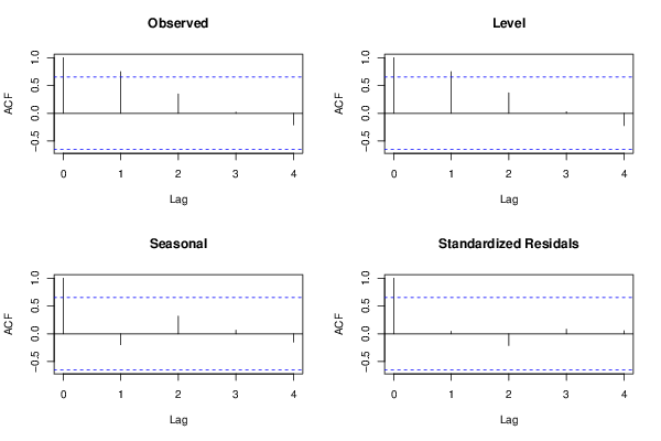
acf(as.numeric(x),lag.max = mylagmax,main='Observed')
acf(mylevel,na.action=na.pass,lag.max = mylagmax,main='Level')
acf(myseas,na.action=na.pass,lag.max = mylagmax,main='Seasonal')
acf(myresid,na.action=na.pass,lag.max = mylagmax,main='Standardized Residals')
par(op)
dev.off()
bitmap(file='test3.png')
op <- par(mfrow = c(2,2))
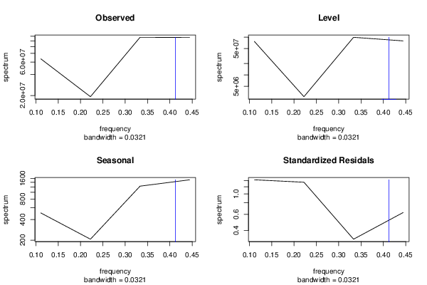
spectrum(as.numeric(x),main='Observed')
spectrum(mylevel,main='Level')
spectrum(myseas,main='Seasonal')
spectrum(myresid,main='Standardized Residals')
par(op)
dev.off()
bitmap(file='test4.png')
op <- par(mfrow = c(2,2))
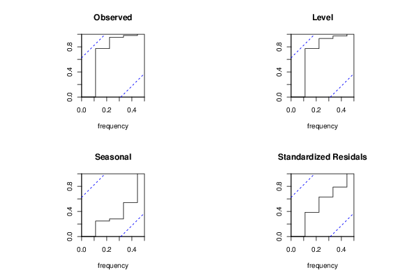
cpgram(as.numeric(x),main='Observed')
cpgram(mylevel,main='Level')
cpgram(myseas,main='Seasonal')
cpgram(myresid,main='Standardized Residals')
par(op)
dev.off()
bitmap(file='test1.png')
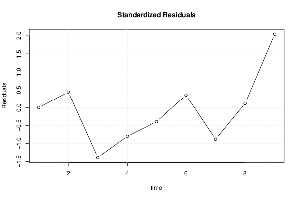
plot(as.numeric(m$resid),main='Standardized Residuals',ylab='Residuals',xlab='time',type='b')
grid()
dev.off()
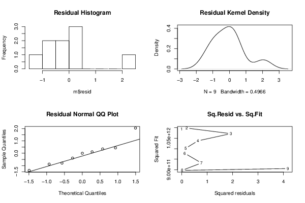
bitmap(file='test5.png')
op <- par(mfrow = c(2,2))
hist(m$resid,main='Residual Histogram')
plot(density(m$resid),main='Residual Kernel Density')
qqnorm(m$resid,main='Residual Normal QQ Plot')
qqline(m$resid)
plot(m$resid^2, myfit^2,main='Sq.Resid vs. Sq.Fit',xlab='Squared residuals',ylab='Squared Fit')
par(op)
dev.off()
load(file='createtable')
a<-table.start()
a<-table.row.start(a)
a<-table.element(a,'Structural Time Series Model',6,TRUE)
a<-table.row.end(a)
a<-table.row.start(a)
a<-table.element(a,'t',header=TRUE)
a<-table.element(a,'Observed',header=TRUE)
a<-table.element(a,'Level',header=TRUE)
a<-table.element(a,'Slope',header=TRUE)
a<-table.element(a,'Seasonal',header=TRUE)
a<-table.element(a,'Stand. Residuals',header=TRUE)
a<-table.row.end(a)
for (i in 1:nx) {
a<-table.row.start(a)
a<-table.element(a,i,header=TRUE)
a<-table.element(a,x[i])
a<-table.element(a,mylevel[i])
a<-table.element(a,myslope[i])
a<-table.element(a,myseas[i])
a<-table.element(a,myresid[i])
a<-table.row.end(a)
}
a<-table.end(a)
table.save(a,file='mytable.tab')