Repository of Reproducible Computations

Free Statistics

of Irreproducible Research!

Author's title

Author

*The author of this computation has been verified*

R Software Module

rwasp_pairs.wasp

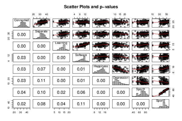
Title produced by software

Kendall tau Correlation Matrix

Date of computation

Wed, 27 Nov 2013 06:40:44 -0500

Cite this page as follows

Statistical Computations at FreeStatistics.org, Office for Research Development and Education, URL https://freestatistics.org/blog/index.php?v=date/2013/Nov/27/t138555266839z1ec4im0ebqxn.htm/, Retrieved Mon, 29 Apr 2024 13:55:33 +0000

Statistical Computations at FreeStatistics.org, Office for Research Development and Education, URL https://freestatistics.org/blog/index.php?pk=228960, Retrieved Mon, 29 Apr 2024 13:55:33 +0000

QR Codes:

Paste this QR Code to cite your computation.

Original text written by user:

IsPrivate?

No (this computation is public)

User-defined keywords

Estimated Impact

112

Family? (F = Feedback message, R = changed R code, M = changed R Module, P = changed Parameters, D = changed Data)

-       [Kendall tau Correlation Matrix] [sm] [2013-11-27 11:40:44] [e931f330ae8eb739e69629b6955c783c] [Current]

Feedback Forum

Post a new message

Dataseries X:

Download CSV

Histogram

Boxplots

41 38 13 12 14 12 53 32
39 32 16 11 18 11 83 51
30 35 19 15 11 14 66 42
31 33 15 6 12 12 67 41
34 37 14 13 16 21 76 46
35 29 13 10 18 12 78 47
39 31 19 12 14 22 53 37
34 36 15 14 14 11 80 49
36 35 14 12 15 10 74 45
37 38 15 9 15 13 76 47
38 31 16 10 17 10 79 49
36 34 16 12 19 8 54 33
38 35 16 12 10 15 67 42
39 38 16 11 16 14 54 33
33 37 17 15 18 10 87 53
32 33 15 12 14 14 58 36
36 32 15 10 14 14 75 45
38 38 20 12 17 11 88 54
39 38 18 11 14 10 64 41
32 32 16 12 16 13 57 36
32 33 16 11 18 9.5 66 41
31 31 16 12 11 14 68 44
39 38 19 13 14 12 54 33
37 39 16 11 12 14 56 37
39 32 17 12 17 11 86 52
41 32 17 13 9 9 80 47
36 35 16 10 16 11 76 43
33 37 15 14 14 15 69 44
33 33 16 12 15 14 78 45
34 33 14 10 11 13 67 44
31 31 15 12 16 9 80 49
27 32 12 8 13 15 54 33
37 31 14 10 17 10 71 43
34 37 16 12 15 11 84 54
34 30 14 12 14 13 74 42
32 33 10 7 16 8 71 44
29 31 10 9 9 20 63 37
36 33 14 12 15 12 71 43
29 31 16 10 17 10 76 46
35 33 16 10 13 10 69 42
37 32 16 10 15 9 74 45
34 33 14 12 16 14 75 44
38 32 20 15 16 8 54 33
35 33 14 10 12 14 52 31
38 28 14 10 15 11 69 42
37 35 11 12 11 13 68 40
38 39 14 13 15 9 65 43
33 34 15 11 15 11 75 46
36 38 16 11 17 15 74 42
38 32 14 12 13 11 75 45
32 38 16 14 16 10 72 44
32 30 14 10 14 14 67 40
32 33 12 12 11 18 63 37
34 38 16 13 12 14 62 46
32 32 9 5 12 11 63 36
37 35 14 6 15 14.5 76 47
39 34 16 12 16 13 74 45
29 34 16 12 15 9 67 42
37 36 15 11 12 10 73 43
35 34 16 10 12 15 70 43
30 28 12 7 8 20 53 32
38 34 16 12 13 12 77 45
34 35 16 14 11 12 80 48
31 35 14 11 14 14 52 31
34 31 16 12 15 13 54 33
35 37 17 13 10 11 80 49
36 35 18 14 11 17 66 42
30 27 18 11 12 12 73 41
39 40 12 12 15 13 63 38
35 37 16 12 15 14 69 42
38 36 10 8 14 13 67 44
31 38 14 11 16 15 54 33
34 39 18 14 15 13 81 48
38 41 18 14 15 10 69 40
34 27 16 12 13 11 84 50
39 30 17 9 12 19 80 49
37 37 16 13 17 13 70 43
34 31 16 11 13 17 69 44
28 31 13 12 15 13 77 47
37 27 16 12 13 9 54 33
33 36 16 12 15 11 79 46
35 37 16 12 15 9 71 45
37 33 15 12 16 12 73 43
32 34 15 11 15 12 72 44
33 31 16 10 14 13 77 47
38 39 14 9 15 13 75 45
33 34 16 12 14 12 69 42
29 32 16 12 13 15 54 33
33 33 15 12 7 22 70 43
31 36 12 9 17 13 73 46
36 32 17 15 13 15 54 33
35 41 16 12 15 13 77 46
32 28 15 12 14 15 82 48
29 30 13 12 13 12.5 80 47
39 36 16 10 16 11 80 47
37 35 16 13 12 16 69 43
35 31 16 9 14 11 78 46
37 34 16 12 17 11 81 48
32 36 14 10 15 10 76 46
38 36 16 14 17 10 76 45
37 35 16 11 12 16 73 45
36 37 20 15 16 12 85 52
32 28 15 11 11 11 66 42
33 39 16 11 15 16 79 47
40 32 13 12 9 19 68 41
38 35 17 12 16 11 76 47
41 39 16 12 15 16 71 43
36 35 16 11 10 15 54 33
43 42 12 7 10 24 46 30
30 34 16 12 15 14 85 52
31 33 16 14 11 15 74 44
32 41 17 11 13 11 88 55
32 33 13 11 14 15 38 11
37 34 12 10 18 12 76 47
37 32 18 13 16 10 86 53
33 40 14 13 14 14 54 33
34 40 14 8 14 13 67 44
33 35 13 11 14 9 69 42
38 36 16 12 14 15 90 55
33 37 13 11 12 15 54 33
31 27 16 13 14 14 76 46
38 39 13 12 15 11 89 54
37 38 16 14 15 8 76 47
36 31 15 13 15 11 73 45
31 33 16 15 13 11 79 47
39 32 15 10 17 8 90 55
44 39 17 11 17 10 74 44
33 36 15 9 19 11 81 53
35 33 12 11 15 13 72 44
32 33 16 10 13 11 71 42
28 32 10 11 9 20 66 40
40 37 16 8 15 10 77 46
27 30 12 11 15 15 65 40
37 38 14 12 15 12 74 46
32 29 15 12 16 14 85 53
28 22 13 9 11 23 54 33
34 35 15 11 14 14 63 42
30 35 11 10 11 16 54 35
35 34 12 8 15 11 64 40
31 35 11 9 13 12 69 41
32 34 16 8 15 10 54 33
30 37 15 9 16 14 84 51
30 35 17 15 14 12 86 53
31 23 16 11 15 12 77 46
40 31 10 8 16 11 89 55
32 27 18 13 16 12 76 47
36 36 13 12 11 13 60 38
32 31 16 12 12 11 75 46
35 32 13 9 9 19 73 46
38 39 10 7 16 12 85 53
42 37 15 13 13 17 79 47
34 38 16 9 16 9 71 41
35 39 16 6 12 12 72 44
38 34 14 8 9 19 69 43
33 31 10 8 13 18 78 51
36 32 17 15 13 15 54 33
32 37 13 6 14 14 69 43
33 36 15 9 19 11 81 53
34 32 16 11 13 9 84 51
32 38 12 8 12 18 84 50
34 36 13 8 13 16 69 46
27 26 13 10 10 24 66 43
31 26 12 8 14 14 81 47
38 33 17 14 16 20 82 50
34 39 15 10 10 18 72 43
24 30 10 8 11 23 54 33
30 33 14 11 14 12 78 48
26 25 11 12 12 14 74 44
34 38 13 12 9 16 82 50
27 37 16 12 9 18 73 41
37 31 12 5 11 20 55 34
36 37 16 12 16 12 72 44
41 35 12 10 9 12 78 47
29 25 9 7 13 17 59 35
36 28 12 12 16 13 72 44
32 35 15 11 13 9 78 44
37 33 12 8 9 16 68 43
30 30 12 9 12 18 69 41
31 31 14 10 16 10 67 41
38 37 12 9 11 14 74 42
36 36 16 12 14 11 54 33
35 30 11 6 13 9 67 41
31 36 19 15 15 11 70 44
38 32 15 12 14 10 80 48
22 28 8 12 16 11 89 55
32 36 16 12 13 19 76 44
36 34 17 11 14 14 74 43
39 31 12 7 15 12 87 52
28 28 11 7 13 14 54 30
32 36 11 5 11 21 61 39
32 36 14 12 11 13 38 11
38 40 16 12 14 10 75 44
32 33 12 3 15 15 69 42
35 37 16 11 11 16 62 41
32 32 13 10 15 14 72 44
37 38 15 12 12 12 70 44
34 31 16 9 14 19 79 48
33 37 16 12 14 15 87 53
33 33 14 9 8 19 62 37
26 32 16 12 13 13 77 44
30 30 16 12 9 17 69 44
24 30 14 10 15 12 69 40
34 31 11 9 17 11 75 42
34 32 12 12 13 14 54 35
33 34 15 8 15 11 72 43
34 36 15 11 15 13 74 45
35 37 16 11 14 12 85 55
35 36 16 12 16 15 52 31
36 33 11 10 13 14 70 44
34 33 15 10 16 12 84 50
34 33 12 12 9 17 64 40
41 44 12 12 16 11 84 53
32 39 15 11 11 18 87 54
30 32 15 8 10 13 79 49
35 35 16 12 11 17 67 40
28 25 14 10 15 13 65 41
33 35 17 11 17 11 85 52
39 34 14 10 14 12 83 52
36 35 13 8 8 22 61 36
36 39 15 12 15 14 82 52
35 33 13 12 11 12 76 46
38 36 14 10 16 12 58 31
33 32 15 12 10 17 72 44
31 32 12 9 15 9 72 44
34 36 13 9 9 21 38 11
32 36 8 6 16 10 78 46
31 32 14 10 19 11 54 33
33 34 14 9 12 12 63 34
34 33 11 9 8 23 66 42
34 35 12 9 11 13 70 43
34 30 13 6 14 12 71 43
33 38 10 10 9 16 67 44
32 34 16 6 15 9 58 36
41 33 18 14 13 17 72 46
34 32 13 10 16 9 72 44
36 31 11 10 11 14 70 43
37 30 4 6 12 17 76 50
36 27 13 12 13 13 50 33
29 31 16 12 10 11 72 43
37 30 10 7 11 12 72 44
27 32 12 8 12 10 88 53
35 35 12 11 8 19 53 34
28 28 10 3 12 16 58 35
35 33 13 6 12 16 66 40
37 31 15 10 15 14 82 53
29 35 12 8 11 20 69 42
32 35 14 9 13 15 68 43
36 32 10 9 14 23 44 29
19 21 12 8 10 20 56 36
21 20 12 9 12 16 53 30
31 34 11 7 15 14 70 42
33 32 10 7 13 17 78 47
36 34 12 6 13 11 71 44
33 32 16 9 13 13 72 45
37 33 12 10 12 17 68 44
34 33 14 11 12 15 67 43
35 37 16 12 9 21 75 43
31 32 14 8 9 18 62 40
37 34 13 11 15 15 67 41
35 30 4 3 10 8 83 52
27 30 15 11 14 12 64 38
34 38 11 12 15 12 68 41
40 36 11 7 7 22 62 39
29 32 14 9 14 12 72 43

Summary of computational transaction
Raw Input	view raw input (R code)
Raw Output	view raw output of R engine
Computing time	8 seconds
R Server	'Herman Ole Andreas Wold' @ wold.wessa.net

\begin{tabular}{lllllllll}
\hline
Summary of computational transaction \tabularnewline
Raw Input & view raw input (R code)  \tabularnewline
Raw Output & view raw output of R engine  \tabularnewline
Computing time & 8 seconds \tabularnewline
R Server & 'Herman Ole Andreas Wold' @ wold.wessa.net \tabularnewline
\hline
\end{tabular}
%Source: https://freestatistics.org/blog/index.php?pk=228960&T=0

[TABLE]
[ROW][C]Summary of computational transaction[/C][/ROW]
[ROW][C]Raw Input[/C][C]view raw input (R code) [/C][/ROW]
[ROW][C]Raw Output[/C][C]view raw output of R engine [/C][/ROW]
[ROW][C]Computing time[/C][C]8 seconds[/C][/ROW]
[ROW][C]R Server[/C][C]'Herman Ole Andreas Wold' @ wold.wessa.net[/C][/ROW]
[/TABLE]
Source: https://freestatistics.org/blog/index.php?pk=228960&T=0

Globally Unique Identifier (entire table): ba.freestatistics.org/blog/index.php?pk=228960&T=0

As an alternative you can also use a QR Code:

The GUIDs for individual cells are displayed in the table below:

Summary of computational transaction
Raw Input	view raw input (R code)
Raw Output	view raw output of R engine
Computing time	8 seconds
R Server	'Herman Ole Andreas Wold' @ wold.wessa.net

Correlations for all pairs of data series (method=pearson)
	Connected	Separate	Learning	Software	Happiness	Depression	Sport1	Sport2
Connected	1	0.455	0.2	0.134	0.133	-0.136	0.124	0.144
Separate	0.455	1	0.223	0.19	0.11	-0.099	0.1	0.107
Learning	0.2	0.223	1	0.623	0.249	-0.231	0.143	0.125
Software	0.134	0.19	0.623	1	0.164	-0.164	0.114	0.098
Happiness	0.133	0.11	0.249	0.164	1	-0.583	0.287	0.263
Depression	-0.136	-0.099	-0.231	-0.164	-0.583	1	-0.329	-0.283
Sport1	0.124	0.1	0.143	0.114	0.287	-0.329	1	0.953
Sport2	0.144	0.107	0.125	0.098	0.263	-0.283	0.953	1

\begin{tabular}{lllllllll}
\hline
Correlations for all pairs of data series (method=pearson) \tabularnewline
  & Connected & Separate & Learning & Software & Happiness & Depression & Sport1 & Sport2 \tabularnewline
Connected & 1 & 0.455 & 0.2 & 0.134 & 0.133 & -0.136 & 0.124 & 0.144 \tabularnewline
Separate & 0.455 & 1 & 0.223 & 0.19 & 0.11 & -0.099 & 0.1 & 0.107 \tabularnewline
Learning & 0.2 & 0.223 & 1 & 0.623 & 0.249 & -0.231 & 0.143 & 0.125 \tabularnewline
Software & 0.134 & 0.19 & 0.623 & 1 & 0.164 & -0.164 & 0.114 & 0.098 \tabularnewline
Happiness & 0.133 & 0.11 & 0.249 & 0.164 & 1 & -0.583 & 0.287 & 0.263 \tabularnewline
Depression & -0.136 & -0.099 & -0.231 & -0.164 & -0.583 & 1 & -0.329 & -0.283 \tabularnewline
Sport1 & 0.124 & 0.1 & 0.143 & 0.114 & 0.287 & -0.329 & 1 & 0.953 \tabularnewline
Sport2 & 0.144 & 0.107 & 0.125 & 0.098 & 0.263 & -0.283 & 0.953 & 1 \tabularnewline
\hline
\end{tabular}
%Source: https://freestatistics.org/blog/index.php?pk=228960&T=1

[TABLE]
[ROW][C]Correlations for all pairs of data series (method=pearson)[/C][/ROW]
[ROW][C] [/C][C]Connected[/C][C]Separate[/C][C]Learning[/C][C]Software[/C][C]Happiness[/C][C]Depression[/C][C]Sport1[/C][C]Sport2[/C][/ROW]
[ROW][C]Connected[/C][C]1[/C][C]0.455[/C][C]0.2[/C][C]0.134[/C][C]0.133[/C][C]-0.136[/C][C]0.124[/C][C]0.144[/C][/ROW]
[ROW][C]Separate[/C][C]0.455[/C][C]1[/C][C]0.223[/C][C]0.19[/C][C]0.11[/C][C]-0.099[/C][C]0.1[/C][C]0.107[/C][/ROW]
[ROW][C]Learning[/C][C]0.2[/C][C]0.223[/C][C]1[/C][C]0.623[/C][C]0.249[/C][C]-0.231[/C][C]0.143[/C][C]0.125[/C][/ROW]
[ROW][C]Software[/C][C]0.134[/C][C]0.19[/C][C]0.623[/C][C]1[/C][C]0.164[/C][C]-0.164[/C][C]0.114[/C][C]0.098[/C][/ROW]
[ROW][C]Happiness[/C][C]0.133[/C][C]0.11[/C][C]0.249[/C][C]0.164[/C][C]1[/C][C]-0.583[/C][C]0.287[/C][C]0.263[/C][/ROW]
[ROW][C]Depression[/C][C]-0.136[/C][C]-0.099[/C][C]-0.231[/C][C]-0.164[/C][C]-0.583[/C][C]1[/C][C]-0.329[/C][C]-0.283[/C][/ROW]
[ROW][C]Sport1[/C][C]0.124[/C][C]0.1[/C][C]0.143[/C][C]0.114[/C][C]0.287[/C][C]-0.329[/C][C]1[/C][C]0.953[/C][/ROW]
[ROW][C]Sport2[/C][C]0.144[/C][C]0.107[/C][C]0.125[/C][C]0.098[/C][C]0.263[/C][C]-0.283[/C][C]0.953[/C][C]1[/C][/ROW]
[/TABLE]
Source: https://freestatistics.org/blog/index.php?pk=228960&T=1

Globally Unique Identifier (entire table): ba.freestatistics.org/blog/index.php?pk=228960&T=1

As an alternative you can also use a QR Code:

The GUIDs for individual cells are displayed in the table below:

Correlations for all pairs of data series (method=pearson)
	Connected	Separate	Learning	Software	Happiness	Depression	Sport1	Sport2
Connected	1	0.455	0.2	0.134	0.133	-0.136	0.124	0.144
Separate	0.455	1	0.223	0.19	0.11	-0.099	0.1	0.107
Learning	0.2	0.223	1	0.623	0.249	-0.231	0.143	0.125
Software	0.134	0.19	0.623	1	0.164	-0.164	0.114	0.098
Happiness	0.133	0.11	0.249	0.164	1	-0.583	0.287	0.263
Depression	-0.136	-0.099	-0.231	-0.164	-0.583	1	-0.329	-0.283
Sport1	0.124	0.1	0.143	0.114	0.287	-0.329	1	0.953
Sport2	0.144	0.107	0.125	0.098	0.263	-0.283	0.953	1

Correlations for all pairs of data series with p-values
pair	Pearson r	Spearman rho	Kendall tau
Connected;Separate	0.4551	0.3388	0.2521
p-value	(0)	(0)	(0)
Connected;Learning	0.1996	0.1815	0.1373
p-value	(0.0011)	(0.0031)	(0.0026)
Connected;Software	0.1339	0.1489	0.111
p-value	(0.0296)	(0.0155)	(0.015)
Connected;Happiness	0.1328	0.1524	0.1127
p-value	(0.031)	(0.0132)	(0.0125)
Connected;Depression	-0.1364	-0.1382	-0.102
p-value	(0.0267)	(0.0247)	(0.0222)
Connected;Sport1	0.1239	0.1269	0.0929
p-value	(0.0443)	(0.0394)	(0.0328)
Connected;Sport2	0.1439	0.1501	0.1089
p-value	(0.0193)	(0.0146)	(0.0133)
Separate;Learning	0.2227	0.2137	0.1602
p-value	(3e-04)	(5e-04)	(5e-04)
Separate;Software	0.1897	0.2002	0.1481
p-value	(0.002)	(0.0011)	(0.0012)
Separate;Happiness	0.1099	0.1155	0.0815
p-value	(0.0747)	(0.061)	(0.0715)
Separate;Depression	-0.0993	-0.0482	-0.0358
p-value	(0.1073)	(0.4351)	(0.4229)
Separate;Sport1	0.1	0.0686	0.0491
p-value	(0.1049)	(0.2666)	(0.2598)
Separate;Sport2	0.1073	0.0848	0.0607
p-value	(0.082)	(0.1693)	(0.1687)
Learning;Software	0.6234	0.5832	0.4726
p-value	(0)	(0)	(0)
Learning;Happiness	0.2486	0.2395	0.1798
p-value	(0)	(1e-04)	(1e-04)
Learning;Depression	-0.2309	-0.2491	-0.1892
p-value	(2e-04)	(0)	(0)
Learning;Sport1	0.1432	0.2203	0.1662
p-value	(0.02)	(3e-04)	(2e-04)
Learning;Sport2	0.125	0.1971	0.1494
p-value	(0.0424)	(0.0013)	(9e-04)
Software;Happiness	0.1642	0.1523	0.1123
p-value	(0.0075)	(0.0132)	(0.0154)
Software;Depression	-0.1636	-0.1296	-0.0961
p-value	(0.0077)	(0.0353)	(0.0361)
Software;Sport1	0.1139	0.1356	0.1001
p-value	(0.0647)	(0.0276)	(0.0253)
Software;Sport2	0.0976	0.1328	0.0985
p-value	(0.1137)	(0.031)	(0.0294)
Happiness;Depression	-0.5829	-0.5407	-0.4228
p-value	(0)	(0)	(0)
Happiness;Sport1	0.2871	0.3321	0.2409
p-value	(0)	(0)	(0)
Happiness;Sport2	0.2633	0.2975	0.2184
p-value	(0)	(0)	(0)
Depression;Sport1	-0.3294	-0.3248	-0.233
p-value	(0)	(0)	(0)
Depression;Sport2	-0.2829	-0.2823	-0.2045
p-value	(0)	(0)	(0)
Sport1;Sport2	0.953	0.9457	0.8488
p-value	(0)	(0)	(0)

\begin{tabular}{lllllllll}
\hline
Correlations for all pairs of data series with p-values \tabularnewline
pair & Pearson r & Spearman rho & Kendall tau \tabularnewline
Connected;Separate & 0.4551 & 0.3388 & 0.2521 \tabularnewline
p-value & (0) & (0) & (0) \tabularnewline
Connected;Learning & 0.1996 & 0.1815 & 0.1373 \tabularnewline
p-value & (0.0011) & (0.0031) & (0.0026) \tabularnewline
Connected;Software & 0.1339 & 0.1489 & 0.111 \tabularnewline
p-value & (0.0296) & (0.0155) & (0.015) \tabularnewline
Connected;Happiness & 0.1328 & 0.1524 & 0.1127 \tabularnewline
p-value & (0.031) & (0.0132) & (0.0125) \tabularnewline
Connected;Depression & -0.1364 & -0.1382 & -0.102 \tabularnewline
p-value & (0.0267) & (0.0247) & (0.0222) \tabularnewline
Connected;Sport1 & 0.1239 & 0.1269 & 0.0929 \tabularnewline
p-value & (0.0443) & (0.0394) & (0.0328) \tabularnewline
Connected;Sport2 & 0.1439 & 0.1501 & 0.1089 \tabularnewline
p-value & (0.0193) & (0.0146) & (0.0133) \tabularnewline
Separate;Learning & 0.2227 & 0.2137 & 0.1602 \tabularnewline
p-value & (3e-04) & (5e-04) & (5e-04) \tabularnewline
Separate;Software & 0.1897 & 0.2002 & 0.1481 \tabularnewline
p-value & (0.002) & (0.0011) & (0.0012) \tabularnewline
Separate;Happiness & 0.1099 & 0.1155 & 0.0815 \tabularnewline
p-value & (0.0747) & (0.061) & (0.0715) \tabularnewline
Separate;Depression & -0.0993 & -0.0482 & -0.0358 \tabularnewline
p-value & (0.1073) & (0.4351) & (0.4229) \tabularnewline
Separate;Sport1 & 0.1 & 0.0686 & 0.0491 \tabularnewline
p-value & (0.1049) & (0.2666) & (0.2598) \tabularnewline
Separate;Sport2 & 0.1073 & 0.0848 & 0.0607 \tabularnewline
p-value & (0.082) & (0.1693) & (0.1687) \tabularnewline
Learning;Software & 0.6234 & 0.5832 & 0.4726 \tabularnewline
p-value & (0) & (0) & (0) \tabularnewline
Learning;Happiness & 0.2486 & 0.2395 & 0.1798 \tabularnewline
p-value & (0) & (1e-04) & (1e-04) \tabularnewline
Learning;Depression & -0.2309 & -0.2491 & -0.1892 \tabularnewline
p-value & (2e-04) & (0) & (0) \tabularnewline
Learning;Sport1 & 0.1432 & 0.2203 & 0.1662 \tabularnewline
p-value & (0.02) & (3e-04) & (2e-04) \tabularnewline
Learning;Sport2 & 0.125 & 0.1971 & 0.1494 \tabularnewline
p-value & (0.0424) & (0.0013) & (9e-04) \tabularnewline
Software;Happiness & 0.1642 & 0.1523 & 0.1123 \tabularnewline
p-value & (0.0075) & (0.0132) & (0.0154) \tabularnewline
Software;Depression & -0.1636 & -0.1296 & -0.0961 \tabularnewline
p-value & (0.0077) & (0.0353) & (0.0361) \tabularnewline
Software;Sport1 & 0.1139 & 0.1356 & 0.1001 \tabularnewline
p-value & (0.0647) & (0.0276) & (0.0253) \tabularnewline
Software;Sport2 & 0.0976 & 0.1328 & 0.0985 \tabularnewline
p-value & (0.1137) & (0.031) & (0.0294) \tabularnewline
Happiness;Depression & -0.5829 & -0.5407 & -0.4228 \tabularnewline
p-value & (0) & (0) & (0) \tabularnewline
Happiness;Sport1 & 0.2871 & 0.3321 & 0.2409 \tabularnewline
p-value & (0) & (0) & (0) \tabularnewline
Happiness;Sport2 & 0.2633 & 0.2975 & 0.2184 \tabularnewline
p-value & (0) & (0) & (0) \tabularnewline
Depression;Sport1 & -0.3294 & -0.3248 & -0.233 \tabularnewline
p-value & (0) & (0) & (0) \tabularnewline
Depression;Sport2 & -0.2829 & -0.2823 & -0.2045 \tabularnewline
p-value & (0) & (0) & (0) \tabularnewline
Sport1;Sport2 & 0.953 & 0.9457 & 0.8488 \tabularnewline
p-value & (0) & (0) & (0) \tabularnewline
\hline
\end{tabular}
%Source: https://freestatistics.org/blog/index.php?pk=228960&T=2

[TABLE]
[ROW][C]Correlations for all pairs of data series with p-values[/C][/ROW]
[ROW][C]pair[/C][C]Pearson r[/C][C]Spearman rho[/C][C]Kendall tau[/C][/ROW]
[ROW][C]Connected;Separate[/C][C]0.4551[/C][C]0.3388[/C][C]0.2521[/C][/ROW]
[ROW][C]p-value[/C][C](0)[/C][C](0)[/C][C](0)[/C][/ROW]
[ROW][C]Connected;Learning[/C][C]0.1996[/C][C]0.1815[/C][C]0.1373[/C][/ROW]
[ROW][C]p-value[/C][C](0.0011)[/C][C](0.0031)[/C][C](0.0026)[/C][/ROW]
[ROW][C]Connected;Software[/C][C]0.1339[/C][C]0.1489[/C][C]0.111[/C][/ROW]
[ROW][C]p-value[/C][C](0.0296)[/C][C](0.0155)[/C][C](0.015)[/C][/ROW]
[ROW][C]Connected;Happiness[/C][C]0.1328[/C][C]0.1524[/C][C]0.1127[/C][/ROW]
[ROW][C]p-value[/C][C](0.031)[/C][C](0.0132)[/C][C](0.0125)[/C][/ROW]
[ROW][C]Connected;Depression[/C][C]-0.1364[/C][C]-0.1382[/C][C]-0.102[/C][/ROW]
[ROW][C]p-value[/C][C](0.0267)[/C][C](0.0247)[/C][C](0.0222)[/C][/ROW]
[ROW][C]Connected;Sport1[/C][C]0.1239[/C][C]0.1269[/C][C]0.0929[/C][/ROW]
[ROW][C]p-value[/C][C](0.0443)[/C][C](0.0394)[/C][C](0.0328)[/C][/ROW]
[ROW][C]Connected;Sport2[/C][C]0.1439[/C][C]0.1501[/C][C]0.1089[/C][/ROW]
[ROW][C]p-value[/C][C](0.0193)[/C][C](0.0146)[/C][C](0.0133)[/C][/ROW]
[ROW][C]Separate;Learning[/C][C]0.2227[/C][C]0.2137[/C][C]0.1602[/C][/ROW]
[ROW][C]p-value[/C][C](3e-04)[/C][C](5e-04)[/C][C](5e-04)[/C][/ROW]
[ROW][C]Separate;Software[/C][C]0.1897[/C][C]0.2002[/C][C]0.1481[/C][/ROW]
[ROW][C]p-value[/C][C](0.002)[/C][C](0.0011)[/C][C](0.0012)[/C][/ROW]
[ROW][C]Separate;Happiness[/C][C]0.1099[/C][C]0.1155[/C][C]0.0815[/C][/ROW]
[ROW][C]p-value[/C][C](0.0747)[/C][C](0.061)[/C][C](0.0715)[/C][/ROW]
[ROW][C]Separate;Depression[/C][C]-0.0993[/C][C]-0.0482[/C][C]-0.0358[/C][/ROW]
[ROW][C]p-value[/C][C](0.1073)[/C][C](0.4351)[/C][C](0.4229)[/C][/ROW]
[ROW][C]Separate;Sport1[/C][C]0.1[/C][C]0.0686[/C][C]0.0491[/C][/ROW]
[ROW][C]p-value[/C][C](0.1049)[/C][C](0.2666)[/C][C](0.2598)[/C][/ROW]
[ROW][C]Separate;Sport2[/C][C]0.1073[/C][C]0.0848[/C][C]0.0607[/C][/ROW]
[ROW][C]p-value[/C][C](0.082)[/C][C](0.1693)[/C][C](0.1687)[/C][/ROW]
[ROW][C]Learning;Software[/C][C]0.6234[/C][C]0.5832[/C][C]0.4726[/C][/ROW]
[ROW][C]p-value[/C][C](0)[/C][C](0)[/C][C](0)[/C][/ROW]
[ROW][C]Learning;Happiness[/C][C]0.2486[/C][C]0.2395[/C][C]0.1798[/C][/ROW]
[ROW][C]p-value[/C][C](0)[/C][C](1e-04)[/C][C](1e-04)[/C][/ROW]
[ROW][C]Learning;Depression[/C][C]-0.2309[/C][C]-0.2491[/C][C]-0.1892[/C][/ROW]
[ROW][C]p-value[/C][C](2e-04)[/C][C](0)[/C][C](0)[/C][/ROW]
[ROW][C]Learning;Sport1[/C][C]0.1432[/C][C]0.2203[/C][C]0.1662[/C][/ROW]
[ROW][C]p-value[/C][C](0.02)[/C][C](3e-04)[/C][C](2e-04)[/C][/ROW]
[ROW][C]Learning;Sport2[/C][C]0.125[/C][C]0.1971[/C][C]0.1494[/C][/ROW]
[ROW][C]p-value[/C][C](0.0424)[/C][C](0.0013)[/C][C](9e-04)[/C][/ROW]
[ROW][C]Software;Happiness[/C][C]0.1642[/C][C]0.1523[/C][C]0.1123[/C][/ROW]
[ROW][C]p-value[/C][C](0.0075)[/C][C](0.0132)[/C][C](0.0154)[/C][/ROW]
[ROW][C]Software;Depression[/C][C]-0.1636[/C][C]-0.1296[/C][C]-0.0961[/C][/ROW]
[ROW][C]p-value[/C][C](0.0077)[/C][C](0.0353)[/C][C](0.0361)[/C][/ROW]
[ROW][C]Software;Sport1[/C][C]0.1139[/C][C]0.1356[/C][C]0.1001[/C][/ROW]
[ROW][C]p-value[/C][C](0.0647)[/C][C](0.0276)[/C][C](0.0253)[/C][/ROW]
[ROW][C]Software;Sport2[/C][C]0.0976[/C][C]0.1328[/C][C]0.0985[/C][/ROW]
[ROW][C]p-value[/C][C](0.1137)[/C][C](0.031)[/C][C](0.0294)[/C][/ROW]
[ROW][C]Happiness;Depression[/C][C]-0.5829[/C][C]-0.5407[/C][C]-0.4228[/C][/ROW]
[ROW][C]p-value[/C][C](0)[/C][C](0)[/C][C](0)[/C][/ROW]
[ROW][C]Happiness;Sport1[/C][C]0.2871[/C][C]0.3321[/C][C]0.2409[/C][/ROW]
[ROW][C]p-value[/C][C](0)[/C][C](0)[/C][C](0)[/C][/ROW]
[ROW][C]Happiness;Sport2[/C][C]0.2633[/C][C]0.2975[/C][C]0.2184[/C][/ROW]
[ROW][C]p-value[/C][C](0)[/C][C](0)[/C][C](0)[/C][/ROW]
[ROW][C]Depression;Sport1[/C][C]-0.3294[/C][C]-0.3248[/C][C]-0.233[/C][/ROW]
[ROW][C]p-value[/C][C](0)[/C][C](0)[/C][C](0)[/C][/ROW]
[ROW][C]Depression;Sport2[/C][C]-0.2829[/C][C]-0.2823[/C][C]-0.2045[/C][/ROW]
[ROW][C]p-value[/C][C](0)[/C][C](0)[/C][C](0)[/C][/ROW]
[ROW][C]Sport1;Sport2[/C][C]0.953[/C][C]0.9457[/C][C]0.8488[/C][/ROW]
[ROW][C]p-value[/C][C](0)[/C][C](0)[/C][C](0)[/C][/ROW]
[/TABLE]
Source: https://freestatistics.org/blog/index.php?pk=228960&T=2

Globally Unique Identifier (entire table): ba.freestatistics.org/blog/index.php?pk=228960&T=2

As an alternative you can also use a QR Code:

The GUIDs for individual cells are displayed in the table below:

Correlations for all pairs of data series with p-values
pair	Pearson r	Spearman rho	Kendall tau
Connected;Separate	0.4551	0.3388	0.2521
p-value	(0)	(0)	(0)
Connected;Learning	0.1996	0.1815	0.1373
p-value	(0.0011)	(0.0031)	(0.0026)
Connected;Software	0.1339	0.1489	0.111
p-value	(0.0296)	(0.0155)	(0.015)
Connected;Happiness	0.1328	0.1524	0.1127
p-value	(0.031)	(0.0132)	(0.0125)
Connected;Depression	-0.1364	-0.1382	-0.102
p-value	(0.0267)	(0.0247)	(0.0222)
Connected;Sport1	0.1239	0.1269	0.0929
p-value	(0.0443)	(0.0394)	(0.0328)
Connected;Sport2	0.1439	0.1501	0.1089
p-value	(0.0193)	(0.0146)	(0.0133)
Separate;Learning	0.2227	0.2137	0.1602
p-value	(3e-04)	(5e-04)	(5e-04)
Separate;Software	0.1897	0.2002	0.1481
p-value	(0.002)	(0.0011)	(0.0012)
Separate;Happiness	0.1099	0.1155	0.0815
p-value	(0.0747)	(0.061)	(0.0715)
Separate;Depression	-0.0993	-0.0482	-0.0358
p-value	(0.1073)	(0.4351)	(0.4229)
Separate;Sport1	0.1	0.0686	0.0491
p-value	(0.1049)	(0.2666)	(0.2598)
Separate;Sport2	0.1073	0.0848	0.0607
p-value	(0.082)	(0.1693)	(0.1687)
Learning;Software	0.6234	0.5832	0.4726
p-value	(0)	(0)	(0)
Learning;Happiness	0.2486	0.2395	0.1798
p-value	(0)	(1e-04)	(1e-04)
Learning;Depression	-0.2309	-0.2491	-0.1892
p-value	(2e-04)	(0)	(0)
Learning;Sport1	0.1432	0.2203	0.1662
p-value	(0.02)	(3e-04)	(2e-04)
Learning;Sport2	0.125	0.1971	0.1494
p-value	(0.0424)	(0.0013)	(9e-04)
Software;Happiness	0.1642	0.1523	0.1123
p-value	(0.0075)	(0.0132)	(0.0154)
Software;Depression	-0.1636	-0.1296	-0.0961
p-value	(0.0077)	(0.0353)	(0.0361)
Software;Sport1	0.1139	0.1356	0.1001
p-value	(0.0647)	(0.0276)	(0.0253)
Software;Sport2	0.0976	0.1328	0.0985
p-value	(0.1137)	(0.031)	(0.0294)
Happiness;Depression	-0.5829	-0.5407	-0.4228
p-value	(0)	(0)	(0)
Happiness;Sport1	0.2871	0.3321	0.2409
p-value	(0)	(0)	(0)
Happiness;Sport2	0.2633	0.2975	0.2184
p-value	(0)	(0)	(0)
Depression;Sport1	-0.3294	-0.3248	-0.233
p-value	(0)	(0)	(0)
Depression;Sport2	-0.2829	-0.2823	-0.2045
p-value	(0)	(0)	(0)
Sport1;Sport2	0.953	0.9457	0.8488
p-value	(0)	(0)	(0)

Meta Analysis of Correlation Tests
Number of significant by total number of Correlations
Type I error	Pearson r	Spearman rho	Kendall tau
0.01	0.54	0.54	0.54
0.02	0.61	0.68	0.68
0.03	0.68	0.75	0.79
0.04	0.71	0.86	0.86
0.05	0.79	0.86	0.86
0.06	0.79	0.86	0.86
0.07	0.82	0.89	0.86
0.08	0.86	0.89	0.89
0.09	0.89	0.89	0.89
0.1	0.89	0.89	0.89

\begin{tabular}{lllllllll}
\hline
Meta Analysis of Correlation Tests \tabularnewline
Number of significant by total number of Correlations \tabularnewline
Type I error & Pearson r & Spearman rho & Kendall tau \tabularnewline
0.01 & 0.54 & 0.54 & 0.54 \tabularnewline
0.02 & 0.61 & 0.68 & 0.68 \tabularnewline
0.03 & 0.68 & 0.75 & 0.79 \tabularnewline
0.04 & 0.71 & 0.86 & 0.86 \tabularnewline
0.05 & 0.79 & 0.86 & 0.86 \tabularnewline
0.06 & 0.79 & 0.86 & 0.86 \tabularnewline
0.07 & 0.82 & 0.89 & 0.86 \tabularnewline
0.08 & 0.86 & 0.89 & 0.89 \tabularnewline
0.09 & 0.89 & 0.89 & 0.89 \tabularnewline
0.1 & 0.89 & 0.89 & 0.89 \tabularnewline
\hline
\end{tabular}
%Source: https://freestatistics.org/blog/index.php?pk=228960&T=3

[TABLE]
[ROW][C]Meta Analysis of Correlation Tests[/C][/ROW]
[ROW][C]Number of significant by total number of Correlations[/C][/ROW]
[ROW][C]Type I error[/C][C]Pearson r[/C][C]Spearman rho[/C][C]Kendall tau[/C][/ROW]
[ROW][C]0.01[/C][C]0.54[/C][C]0.54[/C][C]0.54[/C][/ROW]
[ROW][C]0.02[/C][C]0.61[/C][C]0.68[/C][C]0.68[/C][/ROW]
[ROW][C]0.03[/C][C]0.68[/C][C]0.75[/C][C]0.79[/C][/ROW]
[ROW][C]0.04[/C][C]0.71[/C][C]0.86[/C][C]0.86[/C][/ROW]
[ROW][C]0.05[/C][C]0.79[/C][C]0.86[/C][C]0.86[/C][/ROW]
[ROW][C]0.06[/C][C]0.79[/C][C]0.86[/C][C]0.86[/C][/ROW]
[ROW][C]0.07[/C][C]0.82[/C][C]0.89[/C][C]0.86[/C][/ROW]
[ROW][C]0.08[/C][C]0.86[/C][C]0.89[/C][C]0.89[/C][/ROW]
[ROW][C]0.09[/C][C]0.89[/C][C]0.89[/C][C]0.89[/C][/ROW]
[ROW][C]0.1[/C][C]0.89[/C][C]0.89[/C][C]0.89[/C][/ROW]
[/TABLE]
Source: https://freestatistics.org/blog/index.php?pk=228960&T=3

Globally Unique Identifier (entire table): ba.freestatistics.org/blog/index.php?pk=228960&T=3

As an alternative you can also use a QR Code:

The GUIDs for individual cells are displayed in the table below:

Meta Analysis of Correlation Tests
Number of significant by total number of Correlations
Type I error	Pearson r	Spearman rho	Kendall tau
0.01	0.54	0.54	0.54
0.02	0.61	0.68	0.68
0.03	0.68	0.75	0.79
0.04	0.71	0.86	0.86
0.05	0.79	0.86	0.86
0.06	0.79	0.86	0.86
0.07	0.82	0.89	0.86
0.08	0.86	0.89	0.89
0.09	0.89	0.89	0.89
0.1	0.89	0.89	0.89

Figure 1

PNG link

Postscript link

PDF link

Parameters (Session):

par1 = pearson ;

Parameters (R input):

par1 = pearson ;

R code (references can be found in the software module):

panel.tau <- function(x, y, digits=2, prefix='', cex.cor)
{
usr <- par('usr'); on.exit(par(usr))
par(usr = c(0, 1, 0, 1))
rr <- cor.test(x, y, method=par1)
r <- round(rr$p.value,2)
txt <- format(c(r, 0.123456789), digits=digits)[1]
txt <- paste(prefix, txt, sep='')
if(missing(cex.cor)) cex <- 0.5/strwidth(txt)
text(0.5, 0.5, txt, cex = cex)
}
panel.hist <- function(x, ...)
{
usr <- par('usr'); on.exit(par(usr))
par(usr = c(usr[1:2], 0, 1.5) )
h <- hist(x, plot = FALSE)
breaks <- h$breaks; nB <- length(breaks)
y <- h$counts; y <- y/max(y)
rect(breaks[-nB], 0, breaks[-1], y, col='grey', ...)
}
bitmap(file='test1.png')
pairs(t(y),diag.panel=panel.hist, upper.panel=panel.smooth, lower.panel=panel.tau, main=main)
dev.off()
load(file='createtable')
n <- length(y[,1])
n
a<-table.start()
a<-table.row.start(a)
a<-table.element(a,paste('Correlations for all pairs of data series (method=',par1,')',sep=''),n+1,TRUE)
a<-table.row.end(a)
a<-table.row.start(a)
a<-table.element(a,' ',header=TRUE)
for (i in 1:n) {
a<-table.element(a,dimnames(t(x))[[2]][i],header=TRUE)
}
a<-table.row.end(a)
for (i in 1:n) {
a<-table.row.start(a)
a<-table.element(a,dimnames(t(x))[[2]][i],header=TRUE)
for (j in 1:n) {
r <- cor.test(y[i,],y[j,],method=par1)
a<-table.element(a,round(r$estimate,3))
}
a<-table.row.end(a)
}
a<-table.end(a)
table.save(a,file='mytable.tab')
ncorrs <- (n*n -n)/2
mycorrs <- array(0, dim=c(10,3))
a<-table.start()
a<-table.row.start(a)
a<-table.element(a,'Correlations for all pairs of data series with p-values',4,TRUE)
a<-table.row.end(a)
a<-table.row.start(a)
a<-table.element(a,'pair',1,TRUE)
a<-table.element(a,'Pearson r',1,TRUE)
a<-table.element(a,'Spearman rho',1,TRUE)
a<-table.element(a,'Kendall tau',1,TRUE)
a<-table.row.end(a)
cor.test(y[1,],y[2,],method=par1)
for (i in 1:(n-1))
{
for (j in (i+1):n)
{
a<-table.row.start(a)
dum <- paste(dimnames(t(x))[[2]][i],';',dimnames(t(x))[[2]][j],sep='')
a<-table.element(a,dum,header=TRUE)
rp <- cor.test(y[i,],y[j,],method='pearson')
a<-table.element(a,round(rp$estimate,4))
rs <- cor.test(y[i,],y[j,],method='spearman')
a<-table.element(a,round(rs$estimate,4))
rk <- cor.test(y[i,],y[j,],method='kendall')
a<-table.element(a,round(rk$estimate,4))
a<-table.row.end(a)
a<-table.row.start(a)
a<-table.element(a,'p-value',header=T)
a<-table.element(a,paste('(',round(rp$p.value,4),')',sep=''))
a<-table.element(a,paste('(',round(rs$p.value,4),')',sep=''))
a<-table.element(a,paste('(',round(rk$p.value,4),')',sep=''))
a<-table.row.end(a)
for (iii in 1:10) {
iiid100 <- iii / 100
if (rp$p.value < iiid100) mycorrs[iii, 1] = mycorrs[iii, 1] + 1
if (rs$p.value < iiid100) mycorrs[iii, 2] = mycorrs[iii, 2] + 1
if (rk$p.value < iiid100) mycorrs[iii, 3] = mycorrs[iii, 3] + 1
}
}
}
a<-table.end(a)
table.save(a,file='mytable1.tab')
a<-table.start()
a<-table.row.start(a)
a<-table.element(a,'Meta Analysis of Correlation Tests',4,TRUE)
a<-table.row.end(a)
a<-table.row.start(a)
a<-table.element(a,'Number of significant by total number of Correlations',4,TRUE)
a<-table.row.end(a)
a<-table.row.start(a)
a<-table.element(a,'Type I error',1,TRUE)
a<-table.element(a,'Pearson r',1,TRUE)
a<-table.element(a,'Spearman rho',1,TRUE)
a<-table.element(a,'Kendall tau',1,TRUE)
a<-table.row.end(a)
for (iii in 1:10) {
iiid100 <- iii / 100
a<-table.row.start(a)
a<-table.element(a,round(iiid100,2),header=T)
a<-table.element(a,round(mycorrs[iii,1]/ncorrs,2))
a<-table.element(a,round(mycorrs[iii,2]/ncorrs,2))
a<-table.element(a,round(mycorrs[iii,3]/ncorrs,2))
a<-table.row.end(a)
}
a<-table.end(a)
table.save(a,file='mytable2.tab')

Free Statistics

Description of Statistical Computation

Tree of Dependent Computations

Dataset

Tables (Output of Computation)

Figures (Output of Computation)

Input Parameters & R Code