Free Statistics

of Irreproducible Research!

Author's title

Author*Unverified author*
R Software Modulerwasp_logisticregression.wasp
Title produced by softwareBias-Reduced Logistic Regression
Date of computationMon, 02 Sep 2013 11:28:26 -0400
Cite this page as followsStatistical Computations at FreeStatistics.org, Office for Research Development and Education, URL https://freestatistics.org/blog/index.php?v=date/2013/Sep/02/t1378135737gyl2dafnktdzxe7.htm/, Retrieved Mon, 29 Apr 2024 19:10:06 +0000
Statistical Computations at FreeStatistics.org, Office for Research Development and Education, URL https://freestatistics.org/blog/index.php?pk=211383, Retrieved Mon, 29 Apr 2024 19:10:06 +0000
QR Codes:

Original text written by user:
IsPrivate?No (this computation is public)
User-defined keywords
Estimated Impact181
Family? (F = Feedback message, R = changed R code, M = changed R Module, P = changed Parameters, D = changed Data)
-       [Bias-Reduced Logistic Regression] [] [2013-09-02 15:28:26] [d41d8cd98f00b204e9800998ecf8427e] [Current]
Feedback Forum

Post a new message
Dataseries X:
1	83.33	83.33	100	0	50
0	100	100	0	50	0
0	66.66	83.33	33.33	0	0
1	50	83.33	66.66	0	83.33
0	50	50	33.33	50	0
1	100	100	83.33	83.33	0
1	66.66	50	66.66	50	0


Summary of computational transaction
Raw Inputview raw input (R code)
Raw Outputview raw output of R engine
Computing time3 seconds
R Server'Herman Ole Andreas Wold' @ wold.wessa.net

\begin{tabular}{lllllllll}
\hline
Summary of computational transaction \tabularnewline
Raw Input & view raw input (R code)  \tabularnewline
Raw Output & view raw output of R engine  \tabularnewline
Computing time & 3 seconds \tabularnewline
R Server & 'Herman Ole Andreas Wold' @ wold.wessa.net \tabularnewline
\hline
\end{tabular}
%Source: https://freestatistics.org/blog/index.php?pk=211383&T=0

[TABLE]
[ROW][C]Summary of computational transaction[/C][/ROW]
[ROW][C]Raw Input[/C][C]view raw input (R code) [/C][/ROW]
[ROW][C]Raw Output[/C][C]view raw output of R engine [/C][/ROW]
[ROW][C]Computing time[/C][C]3 seconds[/C][/ROW]
[ROW][C]R Server[/C][C]'Herman Ole Andreas Wold' @ wold.wessa.net[/C][/ROW]
[/TABLE]
Source: https://freestatistics.org/blog/index.php?pk=211383&T=0

Globally Unique Identifier (entire table): ba.freestatistics.org/blog/index.php?pk=211383&T=0

As an alternative you can also use a QR Code:  

The GUIDs for individual cells are displayed in the table below:

Summary of computational transaction
Raw Inputview raw input (R code)
Raw Outputview raw output of R engine
Computing time3 seconds
R Server'Herman Ole Andreas Wold' @ wold.wessa.net


Coefficients of Bias-Reduced Logistic Regression
VariableParameterS.E.t-stat2-sided p-value
(Intercept)-2.143055808308134.00534673907396-0.5350487605484080.687233852863121
X10.03010447498675370.1125962401992050.2673666095199350.833679423002337
X2-0.0233327508231330.0998912463331485-0.2335815367175980.853916574507097
X30.02436393476428330.03807939280583160.6398194133114460.637645531201176
X40.006683586876456760.04464532706036710.1497040634828270.905397976777427
X50.022266693752890.05593384837740330.3980897863964160.758811151474276

\begin{tabular}{lllllllll}
\hline
Coefficients of Bias-Reduced Logistic Regression \tabularnewline
Variable & Parameter & S.E. & t-stat & 2-sided p-value \tabularnewline
(Intercept) & -2.14305580830813 & 4.00534673907396 & -0.535048760548408 & 0.687233852863121 \tabularnewline
X1 & 0.0301044749867537 & 0.112596240199205 & 0.267366609519935 & 0.833679423002337 \tabularnewline
X2 & -0.023332750823133 & 0.0998912463331485 & -0.233581536717598 & 0.853916574507097 \tabularnewline
X3 & 0.0243639347642833 & 0.0380793928058316 & 0.639819413311446 & 0.637645531201176 \tabularnewline
X4 & 0.00668358687645676 & 0.0446453270603671 & 0.149704063482827 & 0.905397976777427 \tabularnewline
X5 & 0.02226669375289 & 0.0559338483774033 & 0.398089786396416 & 0.758811151474276 \tabularnewline
\hline
\end{tabular}
%Source: https://freestatistics.org/blog/index.php?pk=211383&T=1

[TABLE]
[ROW][C]Coefficients of Bias-Reduced Logistic Regression[/C][/ROW]
[ROW][C]Variable[/C][C]Parameter[/C][C]S.E.[/C][C]t-stat[/C][C]2-sided p-value[/C][/ROW]
[ROW][C](Intercept)[/C][C]-2.14305580830813[/C][C]4.00534673907396[/C][C]-0.535048760548408[/C][C]0.687233852863121[/C][/ROW]
[ROW][C]X1[/C][C]0.0301044749867537[/C][C]0.112596240199205[/C][C]0.267366609519935[/C][C]0.833679423002337[/C][/ROW]
[ROW][C]X2[/C][C]-0.023332750823133[/C][C]0.0998912463331485[/C][C]-0.233581536717598[/C][C]0.853916574507097[/C][/ROW]
[ROW][C]X3[/C][C]0.0243639347642833[/C][C]0.0380793928058316[/C][C]0.639819413311446[/C][C]0.637645531201176[/C][/ROW]
[ROW][C]X4[/C][C]0.00668358687645676[/C][C]0.0446453270603671[/C][C]0.149704063482827[/C][C]0.905397976777427[/C][/ROW]
[ROW][C]X5[/C][C]0.02226669375289[/C][C]0.0559338483774033[/C][C]0.398089786396416[/C][C]0.758811151474276[/C][/ROW]
[/TABLE]
Source: https://freestatistics.org/blog/index.php?pk=211383&T=1

Globally Unique Identifier (entire table): ba.freestatistics.org/blog/index.php?pk=211383&T=1

As an alternative you can also use a QR Code:  

The GUIDs for individual cells are displayed in the table below:

Coefficients of Bias-Reduced Logistic Regression
VariableParameterS.E.t-stat2-sided p-value
(Intercept)-2.143055808308134.00534673907396-0.5350487605484080.687233852863121
X10.03010447498675370.1125962401992050.2673666095199350.833679423002337
X2-0.0233327508231330.0998912463331485-0.2335815367175980.853916574507097
X30.02436393476428330.03807939280583160.6398194133114460.637645531201176
X40.006683586876456760.04464532706036710.1497040634828270.905397976777427
X50.022266693752890.05593384837740330.3980897863964160.758811151474276


Summary of Bias-Reduced Logistic Regression
Deviance4.23436844249671
Penalized deviance-27.0390231040697
Residual Degrees of Freedom1
ROC Area1
Hosmer–Lemeshow test
Chi-squareNaN
Degrees of Freedom8
P(>Chi)NaN

\begin{tabular}{lllllllll}
\hline
Summary of Bias-Reduced Logistic Regression \tabularnewline
Deviance & 4.23436844249671 \tabularnewline
Penalized deviance & -27.0390231040697 \tabularnewline
Residual Degrees of Freedom & 1 \tabularnewline
ROC Area & 1 \tabularnewline
Hosmer–Lemeshow test \tabularnewline
Chi-square & NaN \tabularnewline
Degrees of Freedom & 8 \tabularnewline
P(>Chi) & NaN \tabularnewline
\hline
\end{tabular}
%Source: https://freestatistics.org/blog/index.php?pk=211383&T=2

[TABLE]
[ROW][C]Summary of Bias-Reduced Logistic Regression[/C][/ROW]
[ROW][C]Deviance[/C][C]4.23436844249671[/C][/ROW]
[ROW][C]Penalized deviance[/C][C]-27.0390231040697[/C][/ROW]
[ROW][C]Residual Degrees of Freedom[/C][C]1[/C][/ROW]
[ROW][C]ROC Area[/C][C]1[/C][/ROW]
[ROW][C]Hosmer–Lemeshow test[/C][/ROW]
[ROW][C]Chi-square[/C][C]NaN[/C][/ROW]
[ROW][C]Degrees of Freedom[/C][C]8[/C][/ROW]
[ROW][C]P(>Chi)[/C][C]NaN[/C][/ROW]
[/TABLE]
Source: https://freestatistics.org/blog/index.php?pk=211383&T=2

Globally Unique Identifier (entire table): ba.freestatistics.org/blog/index.php?pk=211383&T=2

As an alternative you can also use a QR Code:  

The GUIDs for individual cells are displayed in the table below:

Summary of Bias-Reduced Logistic Regression
Deviance4.23436844249671
Penalized deviance-27.0390231040697
Residual Degrees of Freedom1
ROC Area1
Hosmer–Lemeshow test
Chi-squareNaN
Degrees of Freedom8
P(>Chi)NaN


Fit of Logistic Regression
IndexActualFittedError
110.8777142032440060.122285796755994
200.243846761976123-0.243846761976123
300.219503909773179-0.219503909773179
410.7104217588645860.289578241135414
500.341135012069188-0.341135012069188
610.7542309943693270.245769005630673
710.6582151005814740.341784899418526

\begin{tabular}{lllllllll}
\hline
Fit of Logistic Regression \tabularnewline
Index & Actual & Fitted & Error \tabularnewline
1 & 1 & 0.877714203244006 & 0.122285796755994 \tabularnewline
2 & 0 & 0.243846761976123 & -0.243846761976123 \tabularnewline
3 & 0 & 0.219503909773179 & -0.219503909773179 \tabularnewline
4 & 1 & 0.710421758864586 & 0.289578241135414 \tabularnewline
5 & 0 & 0.341135012069188 & -0.341135012069188 \tabularnewline
6 & 1 & 0.754230994369327 & 0.245769005630673 \tabularnewline
7 & 1 & 0.658215100581474 & 0.341784899418526 \tabularnewline
\hline
\end{tabular}
%Source: https://freestatistics.org/blog/index.php?pk=211383&T=3

[TABLE]
[ROW][C]Fit of Logistic Regression[/C][/ROW]
[ROW][C]Index[/C][C]Actual[/C][C]Fitted[/C][C]Error[/C][/ROW]
[ROW][C]1[/C][C]1[/C][C]0.877714203244006[/C][C]0.122285796755994[/C][/ROW]
[ROW][C]2[/C][C]0[/C][C]0.243846761976123[/C][C]-0.243846761976123[/C][/ROW]
[ROW][C]3[/C][C]0[/C][C]0.219503909773179[/C][C]-0.219503909773179[/C][/ROW]
[ROW][C]4[/C][C]1[/C][C]0.710421758864586[/C][C]0.289578241135414[/C][/ROW]
[ROW][C]5[/C][C]0[/C][C]0.341135012069188[/C][C]-0.341135012069188[/C][/ROW]
[ROW][C]6[/C][C]1[/C][C]0.754230994369327[/C][C]0.245769005630673[/C][/ROW]
[ROW][C]7[/C][C]1[/C][C]0.658215100581474[/C][C]0.341784899418526[/C][/ROW]
[/TABLE]
Source: https://freestatistics.org/blog/index.php?pk=211383&T=3

Globally Unique Identifier (entire table): ba.freestatistics.org/blog/index.php?pk=211383&T=3

As an alternative you can also use a QR Code:  

The GUIDs for individual cells are displayed in the table below:

Fit of Logistic Regression
IndexActualFittedError
110.8777142032440060.122285796755994
200.243846761976123-0.243846761976123
300.219503909773179-0.219503909773179
410.7104217588645860.289578241135414
500.341135012069188-0.341135012069188
610.7542309943693270.245769005630673
710.6582151005814740.341784899418526


Type I & II errors for various threshold values
ThresholdType IType II
0.0101
0.0201
0.0301
0.0401
0.0501
0.0601
0.0701
0.0801
0.0901
0.101
0.1101
0.1201
0.1301
0.1401
0.1501
0.1601
0.1701
0.1801
0.1901
0.201
0.2101
0.2200.666666666666667
0.2300.666666666666667
0.2400.666666666666667
0.2500.333333333333333
0.2600.333333333333333
0.2700.333333333333333
0.2800.333333333333333
0.2900.333333333333333
0.300.333333333333333
0.3100.333333333333333
0.3200.333333333333333
0.3300.333333333333333
0.3400.333333333333333
0.3500
0.3600
0.3700
0.3800
0.3900
0.400
0.4100
0.4200
0.4300
0.4400
0.4500
0.4600
0.4700
0.4800
0.4900
0.500
0.5100
0.5200
0.5300
0.5400
0.5500
0.5600
0.5700
0.5800
0.5900
0.600
0.6100
0.6200
0.6300
0.6400
0.6500
0.660.250
0.670.250
0.680.250
0.690.250
0.70.250
0.710.250
0.720.50
0.730.50
0.740.50
0.750.50
0.760.750
0.770.750
0.780.750
0.790.750
0.80.750
0.810.750
0.820.750
0.830.750
0.840.750
0.850.750
0.860.750
0.870.750
0.8810
0.8910
0.910
0.9110
0.9210
0.9310
0.9410
0.9510
0.9610
0.9710
0.9810
0.9910

\begin{tabular}{lllllllll}
\hline
Type I & II errors for various threshold values \tabularnewline
Threshold & Type I & Type II \tabularnewline
0.01 & 0 & 1 \tabularnewline
0.02 & 0 & 1 \tabularnewline
0.03 & 0 & 1 \tabularnewline
0.04 & 0 & 1 \tabularnewline
0.05 & 0 & 1 \tabularnewline
0.06 & 0 & 1 \tabularnewline
0.07 & 0 & 1 \tabularnewline
0.08 & 0 & 1 \tabularnewline
0.09 & 0 & 1 \tabularnewline
0.1 & 0 & 1 \tabularnewline
0.11 & 0 & 1 \tabularnewline
0.12 & 0 & 1 \tabularnewline
0.13 & 0 & 1 \tabularnewline
0.14 & 0 & 1 \tabularnewline
0.15 & 0 & 1 \tabularnewline
0.16 & 0 & 1 \tabularnewline
0.17 & 0 & 1 \tabularnewline
0.18 & 0 & 1 \tabularnewline
0.19 & 0 & 1 \tabularnewline
0.2 & 0 & 1 \tabularnewline
0.21 & 0 & 1 \tabularnewline
0.22 & 0 & 0.666666666666667 \tabularnewline
0.23 & 0 & 0.666666666666667 \tabularnewline
0.24 & 0 & 0.666666666666667 \tabularnewline
0.25 & 0 & 0.333333333333333 \tabularnewline
0.26 & 0 & 0.333333333333333 \tabularnewline
0.27 & 0 & 0.333333333333333 \tabularnewline
0.28 & 0 & 0.333333333333333 \tabularnewline
0.29 & 0 & 0.333333333333333 \tabularnewline
0.3 & 0 & 0.333333333333333 \tabularnewline
0.31 & 0 & 0.333333333333333 \tabularnewline
0.32 & 0 & 0.333333333333333 \tabularnewline
0.33 & 0 & 0.333333333333333 \tabularnewline
0.34 & 0 & 0.333333333333333 \tabularnewline
0.35 & 0 & 0 \tabularnewline
0.36 & 0 & 0 \tabularnewline
0.37 & 0 & 0 \tabularnewline
0.38 & 0 & 0 \tabularnewline
0.39 & 0 & 0 \tabularnewline
0.4 & 0 & 0 \tabularnewline
0.41 & 0 & 0 \tabularnewline
0.42 & 0 & 0 \tabularnewline
0.43 & 0 & 0 \tabularnewline
0.44 & 0 & 0 \tabularnewline
0.45 & 0 & 0 \tabularnewline
0.46 & 0 & 0 \tabularnewline
0.47 & 0 & 0 \tabularnewline
0.48 & 0 & 0 \tabularnewline
0.49 & 0 & 0 \tabularnewline
0.5 & 0 & 0 \tabularnewline
0.51 & 0 & 0 \tabularnewline
0.52 & 0 & 0 \tabularnewline
0.53 & 0 & 0 \tabularnewline
0.54 & 0 & 0 \tabularnewline
0.55 & 0 & 0 \tabularnewline
0.56 & 0 & 0 \tabularnewline
0.57 & 0 & 0 \tabularnewline
0.58 & 0 & 0 \tabularnewline
0.59 & 0 & 0 \tabularnewline
0.6 & 0 & 0 \tabularnewline
0.61 & 0 & 0 \tabularnewline
0.62 & 0 & 0 \tabularnewline
0.63 & 0 & 0 \tabularnewline
0.64 & 0 & 0 \tabularnewline
0.65 & 0 & 0 \tabularnewline
0.66 & 0.25 & 0 \tabularnewline
0.67 & 0.25 & 0 \tabularnewline
0.68 & 0.25 & 0 \tabularnewline
0.69 & 0.25 & 0 \tabularnewline
0.7 & 0.25 & 0 \tabularnewline
0.71 & 0.25 & 0 \tabularnewline
0.72 & 0.5 & 0 \tabularnewline
0.73 & 0.5 & 0 \tabularnewline
0.74 & 0.5 & 0 \tabularnewline
0.75 & 0.5 & 0 \tabularnewline
0.76 & 0.75 & 0 \tabularnewline
0.77 & 0.75 & 0 \tabularnewline
0.78 & 0.75 & 0 \tabularnewline
0.79 & 0.75 & 0 \tabularnewline
0.8 & 0.75 & 0 \tabularnewline
0.81 & 0.75 & 0 \tabularnewline
0.82 & 0.75 & 0 \tabularnewline
0.83 & 0.75 & 0 \tabularnewline
0.84 & 0.75 & 0 \tabularnewline
0.85 & 0.75 & 0 \tabularnewline
0.86 & 0.75 & 0 \tabularnewline
0.87 & 0.75 & 0 \tabularnewline
0.88 & 1 & 0 \tabularnewline
0.89 & 1 & 0 \tabularnewline
0.9 & 1 & 0 \tabularnewline
0.91 & 1 & 0 \tabularnewline
0.92 & 1 & 0 \tabularnewline
0.93 & 1 & 0 \tabularnewline
0.94 & 1 & 0 \tabularnewline
0.95 & 1 & 0 \tabularnewline
0.96 & 1 & 0 \tabularnewline
0.97 & 1 & 0 \tabularnewline
0.98 & 1 & 0 \tabularnewline
0.99 & 1 & 0 \tabularnewline
\hline
\end{tabular}
%Source: https://freestatistics.org/blog/index.php?pk=211383&T=4

[TABLE]
[ROW][C]Type I & II errors for various threshold values[/C][/ROW]
[ROW][C]Threshold[/C][C]Type I[/C][C]Type II[/C][/ROW]
[ROW][C]0.01[/C][C]0[/C][C]1[/C][/ROW]
[ROW][C]0.02[/C][C]0[/C][C]1[/C][/ROW]
[ROW][C]0.03[/C][C]0[/C][C]1[/C][/ROW]
[ROW][C]0.04[/C][C]0[/C][C]1[/C][/ROW]
[ROW][C]0.05[/C][C]0[/C][C]1[/C][/ROW]
[ROW][C]0.06[/C][C]0[/C][C]1[/C][/ROW]
[ROW][C]0.07[/C][C]0[/C][C]1[/C][/ROW]
[ROW][C]0.08[/C][C]0[/C][C]1[/C][/ROW]
[ROW][C]0.09[/C][C]0[/C][C]1[/C][/ROW]
[ROW][C]0.1[/C][C]0[/C][C]1[/C][/ROW]
[ROW][C]0.11[/C][C]0[/C][C]1[/C][/ROW]
[ROW][C]0.12[/C][C]0[/C][C]1[/C][/ROW]
[ROW][C]0.13[/C][C]0[/C][C]1[/C][/ROW]
[ROW][C]0.14[/C][C]0[/C][C]1[/C][/ROW]
[ROW][C]0.15[/C][C]0[/C][C]1[/C][/ROW]
[ROW][C]0.16[/C][C]0[/C][C]1[/C][/ROW]
[ROW][C]0.17[/C][C]0[/C][C]1[/C][/ROW]
[ROW][C]0.18[/C][C]0[/C][C]1[/C][/ROW]
[ROW][C]0.19[/C][C]0[/C][C]1[/C][/ROW]
[ROW][C]0.2[/C][C]0[/C][C]1[/C][/ROW]
[ROW][C]0.21[/C][C]0[/C][C]1[/C][/ROW]
[ROW][C]0.22[/C][C]0[/C][C]0.666666666666667[/C][/ROW]
[ROW][C]0.23[/C][C]0[/C][C]0.666666666666667[/C][/ROW]
[ROW][C]0.24[/C][C]0[/C][C]0.666666666666667[/C][/ROW]
[ROW][C]0.25[/C][C]0[/C][C]0.333333333333333[/C][/ROW]
[ROW][C]0.26[/C][C]0[/C][C]0.333333333333333[/C][/ROW]
[ROW][C]0.27[/C][C]0[/C][C]0.333333333333333[/C][/ROW]
[ROW][C]0.28[/C][C]0[/C][C]0.333333333333333[/C][/ROW]
[ROW][C]0.29[/C][C]0[/C][C]0.333333333333333[/C][/ROW]
[ROW][C]0.3[/C][C]0[/C][C]0.333333333333333[/C][/ROW]
[ROW][C]0.31[/C][C]0[/C][C]0.333333333333333[/C][/ROW]
[ROW][C]0.32[/C][C]0[/C][C]0.333333333333333[/C][/ROW]
[ROW][C]0.33[/C][C]0[/C][C]0.333333333333333[/C][/ROW]
[ROW][C]0.34[/C][C]0[/C][C]0.333333333333333[/C][/ROW]
[ROW][C]0.35[/C][C]0[/C][C]0[/C][/ROW]
[ROW][C]0.36[/C][C]0[/C][C]0[/C][/ROW]
[ROW][C]0.37[/C][C]0[/C][C]0[/C][/ROW]
[ROW][C]0.38[/C][C]0[/C][C]0[/C][/ROW]
[ROW][C]0.39[/C][C]0[/C][C]0[/C][/ROW]
[ROW][C]0.4[/C][C]0[/C][C]0[/C][/ROW]
[ROW][C]0.41[/C][C]0[/C][C]0[/C][/ROW]
[ROW][C]0.42[/C][C]0[/C][C]0[/C][/ROW]
[ROW][C]0.43[/C][C]0[/C][C]0[/C][/ROW]
[ROW][C]0.44[/C][C]0[/C][C]0[/C][/ROW]
[ROW][C]0.45[/C][C]0[/C][C]0[/C][/ROW]
[ROW][C]0.46[/C][C]0[/C][C]0[/C][/ROW]
[ROW][C]0.47[/C][C]0[/C][C]0[/C][/ROW]
[ROW][C]0.48[/C][C]0[/C][C]0[/C][/ROW]
[ROW][C]0.49[/C][C]0[/C][C]0[/C][/ROW]
[ROW][C]0.5[/C][C]0[/C][C]0[/C][/ROW]
[ROW][C]0.51[/C][C]0[/C][C]0[/C][/ROW]
[ROW][C]0.52[/C][C]0[/C][C]0[/C][/ROW]
[ROW][C]0.53[/C][C]0[/C][C]0[/C][/ROW]
[ROW][C]0.54[/C][C]0[/C][C]0[/C][/ROW]
[ROW][C]0.55[/C][C]0[/C][C]0[/C][/ROW]
[ROW][C]0.56[/C][C]0[/C][C]0[/C][/ROW]
[ROW][C]0.57[/C][C]0[/C][C]0[/C][/ROW]
[ROW][C]0.58[/C][C]0[/C][C]0[/C][/ROW]
[ROW][C]0.59[/C][C]0[/C][C]0[/C][/ROW]
[ROW][C]0.6[/C][C]0[/C][C]0[/C][/ROW]
[ROW][C]0.61[/C][C]0[/C][C]0[/C][/ROW]
[ROW][C]0.62[/C][C]0[/C][C]0[/C][/ROW]
[ROW][C]0.63[/C][C]0[/C][C]0[/C][/ROW]
[ROW][C]0.64[/C][C]0[/C][C]0[/C][/ROW]
[ROW][C]0.65[/C][C]0[/C][C]0[/C][/ROW]
[ROW][C]0.66[/C][C]0.25[/C][C]0[/C][/ROW]
[ROW][C]0.67[/C][C]0.25[/C][C]0[/C][/ROW]
[ROW][C]0.68[/C][C]0.25[/C][C]0[/C][/ROW]
[ROW][C]0.69[/C][C]0.25[/C][C]0[/C][/ROW]
[ROW][C]0.7[/C][C]0.25[/C][C]0[/C][/ROW]
[ROW][C]0.71[/C][C]0.25[/C][C]0[/C][/ROW]
[ROW][C]0.72[/C][C]0.5[/C][C]0[/C][/ROW]
[ROW][C]0.73[/C][C]0.5[/C][C]0[/C][/ROW]
[ROW][C]0.74[/C][C]0.5[/C][C]0[/C][/ROW]
[ROW][C]0.75[/C][C]0.5[/C][C]0[/C][/ROW]
[ROW][C]0.76[/C][C]0.75[/C][C]0[/C][/ROW]
[ROW][C]0.77[/C][C]0.75[/C][C]0[/C][/ROW]
[ROW][C]0.78[/C][C]0.75[/C][C]0[/C][/ROW]
[ROW][C]0.79[/C][C]0.75[/C][C]0[/C][/ROW]
[ROW][C]0.8[/C][C]0.75[/C][C]0[/C][/ROW]
[ROW][C]0.81[/C][C]0.75[/C][C]0[/C][/ROW]
[ROW][C]0.82[/C][C]0.75[/C][C]0[/C][/ROW]
[ROW][C]0.83[/C][C]0.75[/C][C]0[/C][/ROW]
[ROW][C]0.84[/C][C]0.75[/C][C]0[/C][/ROW]
[ROW][C]0.85[/C][C]0.75[/C][C]0[/C][/ROW]
[ROW][C]0.86[/C][C]0.75[/C][C]0[/C][/ROW]
[ROW][C]0.87[/C][C]0.75[/C][C]0[/C][/ROW]
[ROW][C]0.88[/C][C]1[/C][C]0[/C][/ROW]
[ROW][C]0.89[/C][C]1[/C][C]0[/C][/ROW]
[ROW][C]0.9[/C][C]1[/C][C]0[/C][/ROW]
[ROW][C]0.91[/C][C]1[/C][C]0[/C][/ROW]
[ROW][C]0.92[/C][C]1[/C][C]0[/C][/ROW]
[ROW][C]0.93[/C][C]1[/C][C]0[/C][/ROW]
[ROW][C]0.94[/C][C]1[/C][C]0[/C][/ROW]
[ROW][C]0.95[/C][C]1[/C][C]0[/C][/ROW]
[ROW][C]0.96[/C][C]1[/C][C]0[/C][/ROW]
[ROW][C]0.97[/C][C]1[/C][C]0[/C][/ROW]
[ROW][C]0.98[/C][C]1[/C][C]0[/C][/ROW]
[ROW][C]0.99[/C][C]1[/C][C]0[/C][/ROW]
[/TABLE]
Source: https://freestatistics.org/blog/index.php?pk=211383&T=4

Globally Unique Identifier (entire table): ba.freestatistics.org/blog/index.php?pk=211383&T=4

As an alternative you can also use a QR Code:  

The GUIDs for individual cells are displayed in the table below:

Type I & II errors for various threshold values
ThresholdType IType II
0.0101
0.0201
0.0301
0.0401
0.0501
0.0601
0.0701
0.0801
0.0901
0.101
0.1101
0.1201
0.1301
0.1401
0.1501
0.1601
0.1701
0.1801
0.1901
0.201
0.2101
0.2200.666666666666667
0.2300.666666666666667
0.2400.666666666666667
0.2500.333333333333333
0.2600.333333333333333
0.2700.333333333333333
0.2800.333333333333333
0.2900.333333333333333
0.300.333333333333333
0.3100.333333333333333
0.3200.333333333333333
0.3300.333333333333333
0.3400.333333333333333
0.3500
0.3600
0.3700
0.3800
0.3900
0.400
0.4100
0.4200
0.4300
0.4400
0.4500
0.4600
0.4700
0.4800
0.4900
0.500
0.5100
0.5200
0.5300
0.5400
0.5500
0.5600
0.5700
0.5800
0.5900
0.600
0.6100
0.6200
0.6300
0.6400
0.6500
0.660.250
0.670.250
0.680.250
0.690.250
0.70.250
0.710.250
0.720.50
0.730.50
0.740.50
0.750.50
0.760.750
0.770.750
0.780.750
0.790.750
0.80.750
0.810.750
0.820.750
0.830.750
0.840.750
0.850.750
0.860.750
0.870.750
0.8810
0.8910
0.910
0.9110
0.9210
0.9310
0.9410
0.9510
0.9610
0.9710
0.9810
0.9910


Parameters (Session):
Parameters (R input):
R code (references can be found in the software module):
library(brglm)
roc.plot <- function (sd, sdc, newplot = TRUE, ...)
{
sall <- sort(c(sd, sdc))
sens <- 0
specc <- 0
for (i in length(sall):1) {
sens <- c(sens, mean(sd >= sall[i], na.rm = T))
specc <- c(specc, mean(sdc >= sall[i], na.rm = T))
}
if (newplot) {
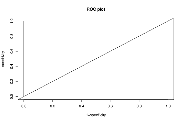
plot(specc, sens, xlim = c(0, 1), ylim = c(0, 1), type = 'l',
xlab = '1-specificity', ylab = 'sensitivity', main = 'ROC plot', ...)
abline(0, 1)
}
else lines(specc, sens, ...)
npoints <- length(sens)
area <- sum(0.5 * (sens[-1] + sens[-npoints]) * (specc[-1] -
specc[-npoints]))
lift <- (sens - specc)[-1]
cutoff <- sall[lift == max(lift)][1]
sensopt <- sens[-1][lift == max(lift)][1]
specopt <- 1 - specc[-1][lift == max(lift)][1]
list(area = area, cutoff = cutoff, sensopt = sensopt, specopt = specopt)
}
roc.analysis <- function (object, newdata = NULL, newplot = TRUE, ...)
{
if (is.null(newdata)) {
sd <- object$fitted[object$y == 1]
sdc <- object$fitted[object$y == 0]
}
else {
sd <- predict(object, newdata, type = 'response')[newdata$y ==
1]
sdc <- predict(object, newdata, type = 'response')[newdata$y ==
0]
}
roc.plot(sd, sdc, newplot, ...)
}
hosmerlem <- function (y, yhat, g = 10)
{
cutyhat <- cut(yhat, breaks = quantile(yhat, probs = seq(0,
1, 1/g)), include.lowest = T)
obs <- xtabs(cbind(1 - y, y) ~ cutyhat)
expect <- xtabs(cbind(1 - yhat, yhat) ~ cutyhat)
chisq <- sum((obs - expect)^2/expect)
P <- 1 - pchisq(chisq, g - 2)
c('X^2' = chisq, Df = g - 2, 'P(>Chi)' = P)
}
x <- as.data.frame(t(y))
r <- brglm(x)
summary(r)
rc <- summary(r)$coeff
try(hm <- hosmerlem(y[1,],r$fitted.values),silent=T)
try(hm,silent=T)
bitmap(file='test0.png')
ra <- roc.analysis(r)
dev.off()
te <- array(0,dim=c(2,99))
for (i in 1:99) {
threshold <- i / 100
numcorr1 <- 0
numfaul1 <- 0
numcorr0 <- 0
numfaul0 <- 0
for (j in 1:length(r$fitted.values)) {
if (y[1,j] > 0.99) {
if (r$fitted.values[j] >= threshold) numcorr1 = numcorr1 + 1 else numfaul1 = numfaul1 + 1
} else {
if (r$fitted.values[j] < threshold) numcorr0 = numcorr0 + 1 else numfaul0 = numfaul0 + 1
}
}
te[1,i] <- numfaul1 / (numfaul1 + numcorr1)
te[2,i] <- numfaul0 / (numfaul0 + numcorr0)
}
bitmap(file='test1.png')
op <- par(mfrow=c(2,2))
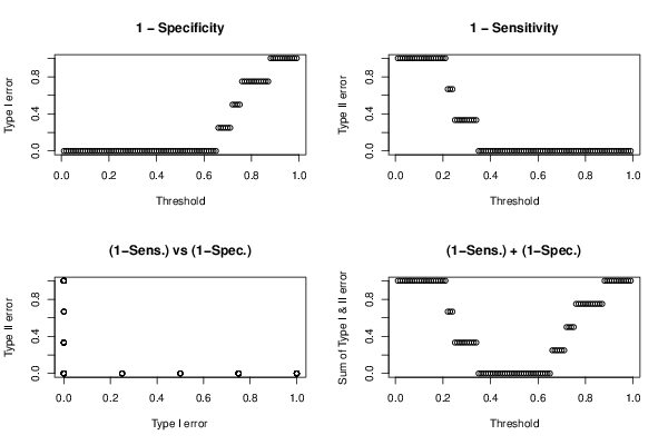
plot((1:99)/100,te[1,],xlab='Threshold',ylab='Type I error', main='1 - Specificity')
plot((1:99)/100,te[2,],xlab='Threshold',ylab='Type II error', main='1 - Sensitivity')
plot(te[1,],te[2,],xlab='Type I error',ylab='Type II error', main='(1-Sens.) vs (1-Spec.)')
plot((1:99)/100,te[1,]+te[2,],xlab='Threshold',ylab='Sum of Type I & II error', main='(1-Sens.) + (1-Spec.)')
par(op)
dev.off()
load(file='createtable')
a<-table.start()
a<-table.row.start(a)
a<-table.element(a,'Coefficients of Bias-Reduced Logistic Regression',5,TRUE)
a<-table.row.end(a)
a<-table.row.start(a)
a<-table.element(a,'Variable',header=TRUE)
a<-table.element(a,'Parameter',header=TRUE)
a<-table.element(a,'S.E.',header=TRUE)
a<-table.element(a,'t-stat',header=TRUE)
a<-table.element(a,'2-sided p-value',header=TRUE)
a<-table.row.end(a)
for (i in 1:length(rc[,1])) {
a<-table.row.start(a)
a<-table.element(a,labels(rc)[[1]][i],header=TRUE)
a<-table.element(a,rc[i,1])
a<-table.element(a,rc[i,2])
a<-table.element(a,rc[i,3])
a<-table.element(a,2*(1-pt(abs(rc[i,3]),r$df.residual)))
a<-table.row.end(a)
}
a<-table.end(a)
table.save(a,file='mytable.tab')
a<-table.start()
a<-table.row.start(a)
a<-table.element(a,'Summary of Bias-Reduced Logistic Regression',2,TRUE)
a<-table.row.end(a)
a<-table.row.start(a)
a<-table.element(a,'Deviance',1,TRUE)
a<-table.element(a,r$deviance)
a<-table.row.end(a)
a<-table.row.start(a)
a<-table.element(a,'Penalized deviance',1,TRUE)
a<-table.element(a,r$penalized.deviance)
a<-table.row.end(a)
a<-table.row.start(a)
a<-table.element(a,'Residual Degrees of Freedom',1,TRUE)
a<-table.element(a,r$df.residual)
a<-table.row.end(a)
a<-table.row.start(a)
a<-table.element(a,'ROC Area',1,TRUE)
a<-table.element(a,ra$area)
a<-table.row.end(a)
a<-table.row.start(a)
a<-table.element(a,'Hosmer–Lemeshow test',2,TRUE)
a<-table.row.end(a)
a<-table.row.start(a)
a<-table.element(a,'Chi-square',1,TRUE)
phm <- array('NA',dim=3)
for (i in 1:3) { try(phm[i] <- hm[i],silent=T) }
a<-table.element(a,phm[1])
a<-table.row.end(a)
a<-table.row.start(a)
a<-table.element(a,'Degrees of Freedom',1,TRUE)
a<-table.element(a,phm[2])
a<-table.row.end(a)
a<-table.row.start(a)
a<-table.element(a,'P(>Chi)',1,TRUE)
a<-table.element(a,phm[3])
a<-table.row.end(a)
a<-table.end(a)
table.save(a,file='mytable1.tab')
a<-table.start()
a<-table.row.start(a)
a<-table.element(a,'Fit of Logistic Regression',4,TRUE)
a<-table.row.end(a)
a<-table.row.start(a)
a<-table.element(a,'Index',1,TRUE)
a<-table.element(a,'Actual',1,TRUE)
a<-table.element(a,'Fitted',1,TRUE)
a<-table.element(a,'Error',1,TRUE)
a<-table.row.end(a)
for (i in 1:length(r$fitted.values)) {
a<-table.row.start(a)
a<-table.element(a,i,1,TRUE)
a<-table.element(a,y[1,i])
a<-table.element(a,r$fitted.values[i])
a<-table.element(a,y[1,i]-r$fitted.values[i])
a<-table.row.end(a)
}
a<-table.end(a)
table.save(a,file='mytable2.tab')
a<-table.start()
a<-table.row.start(a)
a<-table.element(a,'Type I & II errors for various threshold values',3,TRUE)
a<-table.row.end(a)
a<-table.row.start(a)
a<-table.element(a,'Threshold',1,TRUE)
a<-table.element(a,'Type I',1,TRUE)
a<-table.element(a,'Type II',1,TRUE)
a<-table.row.end(a)
for (i in 1:99) {
a<-table.row.start(a)
a<-table.element(a,i/100,1,TRUE)
a<-table.element(a,te[1,i])
a<-table.element(a,te[2,i])
a<-table.row.end(a)
}
a<-table.end(a)
table.save(a,file='mytable3.tab')