Free Statistics
of Irreproducible Research!
Description of Statistical Computation | |||||||||||||||||||||||||||||||||||||||||||||||||||||||||||||||||||||||||||||||||||||||||||||||||||||||||||||||||||||||||||||||||||||||||||||||||||||||||||||||||||||||||||||||||
|---|---|---|---|---|---|---|---|---|---|---|---|---|---|---|---|---|---|---|---|---|---|---|---|---|---|---|---|---|---|---|---|---|---|---|---|---|---|---|---|---|---|---|---|---|---|---|---|---|---|---|---|---|---|---|---|---|---|---|---|---|---|---|---|---|---|---|---|---|---|---|---|---|---|---|---|---|---|---|---|---|---|---|---|---|---|---|---|---|---|---|---|---|---|---|---|---|---|---|---|---|---|---|---|---|---|---|---|---|---|---|---|---|---|---|---|---|---|---|---|---|---|---|---|---|---|---|---|---|---|---|---|---|---|---|---|---|---|---|---|---|---|---|---|---|---|---|---|---|---|---|---|---|---|---|---|---|---|---|---|---|---|---|---|---|---|---|---|---|---|---|---|---|---|---|---|---|---|
| Author's title | |||||||||||||||||||||||||||||||||||||||||||||||||||||||||||||||||||||||||||||||||||||||||||||||||||||||||||||||||||||||||||||||||||||||||||||||||||||||||||||||||||||||||||||||||
| Author | *The author of this computation has been verified* | ||||||||||||||||||||||||||||||||||||||||||||||||||||||||||||||||||||||||||||||||||||||||||||||||||||||||||||||||||||||||||||||||||||||||||||||||||||||||||||||||||||||||||||||||
| R Software Module | rwasp_twosampletests_mean.wasp | ||||||||||||||||||||||||||||||||||||||||||||||||||||||||||||||||||||||||||||||||||||||||||||||||||||||||||||||||||||||||||||||||||||||||||||||||||||||||||||||||||||||||||||||||
| Title produced by software | Paired and Unpaired Two Samples Tests about the Mean | ||||||||||||||||||||||||||||||||||||||||||||||||||||||||||||||||||||||||||||||||||||||||||||||||||||||||||||||||||||||||||||||||||||||||||||||||||||||||||||||||||||||||||||||||
| Date of computation | Sat, 06 Dec 2014 15:44:14 +0000 | ||||||||||||||||||||||||||||||||||||||||||||||||||||||||||||||||||||||||||||||||||||||||||||||||||||||||||||||||||||||||||||||||||||||||||||||||||||||||||||||||||||||||||||||||
| Cite this page as follows | Statistical Computations at FreeStatistics.org, Office for Research Development and Education, URL https://freestatistics.org/blog/index.php?v=date/2014/Dec/06/t1417880726rbfu529nlocj8ol.htm/, Retrieved Thu, 16 May 2024 12:08:24 +0000 | ||||||||||||||||||||||||||||||||||||||||||||||||||||||||||||||||||||||||||||||||||||||||||||||||||||||||||||||||||||||||||||||||||||||||||||||||||||||||||||||||||||||||||||||||
| Statistical Computations at FreeStatistics.org, Office for Research Development and Education, URL https://freestatistics.org/blog/index.php?pk=263648, Retrieved Thu, 16 May 2024 12:08:24 +0000 | |||||||||||||||||||||||||||||||||||||||||||||||||||||||||||||||||||||||||||||||||||||||||||||||||||||||||||||||||||||||||||||||||||||||||||||||||||||||||||||||||||||||||||||||||
| QR Codes: | |||||||||||||||||||||||||||||||||||||||||||||||||||||||||||||||||||||||||||||||||||||||||||||||||||||||||||||||||||||||||||||||||||||||||||||||||||||||||||||||||||||||||||||||||
|
| |||||||||||||||||||||||||||||||||||||||||||||||||||||||||||||||||||||||||||||||||||||||||||||||||||||||||||||||||||||||||||||||||||||||||||||||||||||||||||||||||||||||||||||||||
| Original text written by user: | |||||||||||||||||||||||||||||||||||||||||||||||||||||||||||||||||||||||||||||||||||||||||||||||||||||||||||||||||||||||||||||||||||||||||||||||||||||||||||||||||||||||||||||||||
| IsPrivate? | No (this computation is public) | ||||||||||||||||||||||||||||||||||||||||||||||||||||||||||||||||||||||||||||||||||||||||||||||||||||||||||||||||||||||||||||||||||||||||||||||||||||||||||||||||||||||||||||||||
| User-defined keywords | |||||||||||||||||||||||||||||||||||||||||||||||||||||||||||||||||||||||||||||||||||||||||||||||||||||||||||||||||||||||||||||||||||||||||||||||||||||||||||||||||||||||||||||||||
| Estimated Impact | 118 | ||||||||||||||||||||||||||||||||||||||||||||||||||||||||||||||||||||||||||||||||||||||||||||||||||||||||||||||||||||||||||||||||||||||||||||||||||||||||||||||||||||||||||||||||
Tree of Dependent Computations | |||||||||||||||||||||||||||||||||||||||||||||||||||||||||||||||||||||||||||||||||||||||||||||||||||||||||||||||||||||||||||||||||||||||||||||||||||||||||||||||||||||||||||||||||
| Family? (F = Feedback message, R = changed R code, M = changed R Module, P = changed Parameters, D = changed Data) | |||||||||||||||||||||||||||||||||||||||||||||||||||||||||||||||||||||||||||||||||||||||||||||||||||||||||||||||||||||||||||||||||||||||||||||||||||||||||||||||||||||||||||||||||
| - [Cronbach Alpha] [Intrinsic Motivat...] [2010-10-12 11:42:57] [b98453cac15ba1066b407e146608df68] - RMPD [Survey Scores] [] [2014-10-14 11:37:37] [cc401d1001c65f55a3dfc6f2420e9570] - RMPD [Paired and Unpaired Two Samples Tests about the Mean] [Totale motivatie ...] [2014-12-06 15:44:14] [4ce2356216df8db4950cd852fec912aa] [Current] - RM D [Chi-Squared Test, McNemar Test, and Fisher Exact Test] [Chisquaredtest] [2014-12-06 17:04:15] [5c51c91cab622bcf955f01721b682696] - RM D [Chi-Squared Test, McNemar Test, and Fisher Exact Test] [Chisquaredtest] [2014-12-06 17:13:53] [5c51c91cab622bcf955f01721b682696] - RM D [Chi-Squared Test, McNemar Test, and Fisher Exact Test] [Chisquaredtest] [2014-12-06 17:16:18] [5c51c91cab622bcf955f01721b682696] - RM D [Chi-Squared Test, McNemar Test, and Fisher Exact Test] [Chisquaredtest] [2014-12-06 17:32:28] [5c51c91cab622bcf955f01721b682696] - RM D [Chi-Squared Test, McNemar Test, and Fisher Exact Test] [Chisquaredtest] [2014-12-06 17:36:41] [5c51c91cab622bcf955f01721b682696] | |||||||||||||||||||||||||||||||||||||||||||||||||||||||||||||||||||||||||||||||||||||||||||||||||||||||||||||||||||||||||||||||||||||||||||||||||||||||||||||||||||||||||||||||||
| Feedback Forum | |||||||||||||||||||||||||||||||||||||||||||||||||||||||||||||||||||||||||||||||||||||||||||||||||||||||||||||||||||||||||||||||||||||||||||||||||||||||||||||||||||||||||||||||||
Post a new message | |||||||||||||||||||||||||||||||||||||||||||||||||||||||||||||||||||||||||||||||||||||||||||||||||||||||||||||||||||||||||||||||||||||||||||||||||||||||||||||||||||||||||||||||||
Dataset | |||||||||||||||||||||||||||||||||||||||||||||||||||||||||||||||||||||||||||||||||||||||||||||||||||||||||||||||||||||||||||||||||||||||||||||||||||||||||||||||||||||||||||||||||
| Dataseries X: | |||||||||||||||||||||||||||||||||||||||||||||||||||||||||||||||||||||||||||||||||||||||||||||||||||||||||||||||||||||||||||||||||||||||||||||||||||||||||||||||||||||||||||||||||
72 50 61 68 68 62 61 54 64 71 65 54 69 65 63 73 75 52 63 84 73 42 75 66 63 65 63 78 62 73 64 75 60 66 56 70 59 81 68 71 66 69 73 71 72 72 71 68 59 70 64 67 66 76 78 70 68 60 73 77 62 72 65 69 68 71 65 62 60 70 71 58 65 76 68 52 64 59 74 68 69 76 76 67 68 59 72 76 67 60 63 63 59 70 73 66 66 64 62 70 69 75 66 61 57 60 56 73 71 61 56 66 62 59 59 64 57 66 66 78 63 53 69 67 48 66 66 71 73 51 67 56 61 67 68 69 75 55 62 63 69 67 74 65 63 47 58 76 58 64 72 68 62 64 62 65 65 63 69 60 66 68 72 72 62 70 75 61 58 61 66 62 55 71 47 71 62 51 64 70 64 73 50 76 70 59 69 68 48 48 66 52 73 59 74 60 66 59 78 57 60 79 69 60 65 60 78 59 63 61 71 71 80 58 73 59 69 58 84 60 64 55 58 62 59 69 78 68 67 72 60 19 66 68 74 79 72 71 55 71 49 74 74 75 53 53 64 50 65 70 57 78 51 59 80 72 67 70 70 63 74 74 75 67 70 66 69 62 65 73 71 67 65 61 68 74 67 32 66 69 59 60 72 57 52 60 65 68 68 68 67 73 73 69 65 65 75 81 57 55 62 69 59 48 63 69 73 68 55 74 64 67 78 65 60 63 66 74 68 39 78 68 60 69 64 63 72 70 71 68 80 70 74 78 69 59 75 62 73 75 60 74 76 73 53 62 78 69 67 65 59 67 73 73 70 52 59 61 76 53 66 63 64 78 72 65 57 77 74 69 66 68 74 76 71 63 65 41 70 76 66 67 77 69 72 73 65 63 67 78 72 56 58 56 84 64 63 68 58 75 69 55 80 66 67 75 75 77 71 61 72 71 75 72 79 66 76 66 81 63 60 60 67 64 72 74 79 71 40 69 70 77 66 70 66 77 73 68 74 65 70 69 50 50 64 72 77 64 NA 76 NA 79 NA 55 NA 62 NA 69 NA 68 NA 75 NA 64 NA 63 NA 67 NA 58 NA 71 NA 79 NA 53 NA 57 NA 67 NA 58 NA 74 NA 62 NA 54 NA 62 NA 64 NA 66 NA 66 NA 63 NA 66 NA 78 NA 84 NA 67 NA 58 NA 75 NA 55 NA 72 NA 54 NA 58 NA 67 NA 77 NA 72 NA 52 NA 76 NA 72 NA 77 NA 64 NA 71 NA 73 NA 75 NA 58 NA 51 NA 75 NA 71 | |||||||||||||||||||||||||||||||||||||||||||||||||||||||||||||||||||||||||||||||||||||||||||||||||||||||||||||||||||||||||||||||||||||||||||||||||||||||||||||||||||||||||||||||||
Tables (Output of Computation) | |||||||||||||||||||||||||||||||||||||||||||||||||||||||||||||||||||||||||||||||||||||||||||||||||||||||||||||||||||||||||||||||||||||||||||||||||||||||||||||||||||||||||||||||||
| |||||||||||||||||||||||||||||||||||||||||||||||||||||||||||||||||||||||||||||||||||||||||||||||||||||||||||||||||||||||||||||||||||||||||||||||||||||||||||||||||||||||||||||||||
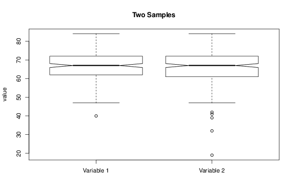
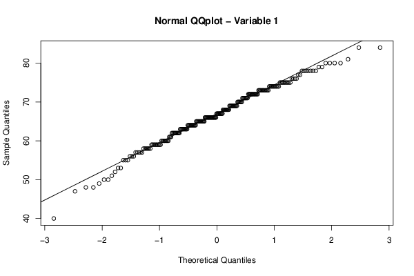
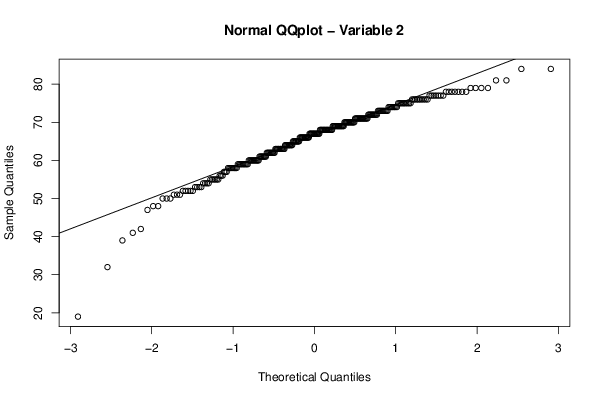
Figures (Output of Computation) | |||||||||||||||||||||||||||||||||||||||||||||||||||||||||||||||||||||||||||||||||||||||||||||||||||||||||||||||||||||||||||||||||||||||||||||||||||||||||||||||||||||||||||||||||
Input Parameters & R Code | |||||||||||||||||||||||||||||||||||||||||||||||||||||||||||||||||||||||||||||||||||||||||||||||||||||||||||||||||||||||||||||||||||||||||||||||||||||||||||||||||||||||||||||||||
| Parameters (Session): | |||||||||||||||||||||||||||||||||||||||||||||||||||||||||||||||||||||||||||||||||||||||||||||||||||||||||||||||||||||||||||||||||||||||||||||||||||||||||||||||||||||||||||||||||
| par1 = black ; | |||||||||||||||||||||||||||||||||||||||||||||||||||||||||||||||||||||||||||||||||||||||||||||||||||||||||||||||||||||||||||||||||||||||||||||||||||||||||||||||||||||||||||||||||
| Parameters (R input): | |||||||||||||||||||||||||||||||||||||||||||||||||||||||||||||||||||||||||||||||||||||||||||||||||||||||||||||||||||||||||||||||||||||||||||||||||||||||||||||||||||||||||||||||||
| par1 = 1 ; par2 = 2 ; par3 = 0.95 ; par4 = two.sided ; par5 = unpaired ; par6 = 0.0 ; | |||||||||||||||||||||||||||||||||||||||||||||||||||||||||||||||||||||||||||||||||||||||||||||||||||||||||||||||||||||||||||||||||||||||||||||||||||||||||||||||||||||||||||||||||
| R code (references can be found in the software module): | |||||||||||||||||||||||||||||||||||||||||||||||||||||||||||||||||||||||||||||||||||||||||||||||||||||||||||||||||||||||||||||||||||||||||||||||||||||||||||||||||||||||||||||||||
par1 <- as.numeric(par1) #column number of first sample | |||||||||||||||||||||||||||||||||||||||||||||||||||||||||||||||||||||||||||||||||||||||||||||||||||||||||||||||||||||||||||||||||||||||||||||||||||||||||||||||||||||||||||||||||