Free Statistics
of Irreproducible Research!
Description of Statistical Computation | |||||||||||||||||||||||||||||||||||||||||||||||||||||||||||||||||||||||||||||||||||||||||||||||||||||||||||||||||||||||||||||||||||||||||||||||||||||||||||||||||||||||||
|---|---|---|---|---|---|---|---|---|---|---|---|---|---|---|---|---|---|---|---|---|---|---|---|---|---|---|---|---|---|---|---|---|---|---|---|---|---|---|---|---|---|---|---|---|---|---|---|---|---|---|---|---|---|---|---|---|---|---|---|---|---|---|---|---|---|---|---|---|---|---|---|---|---|---|---|---|---|---|---|---|---|---|---|---|---|---|---|---|---|---|---|---|---|---|---|---|---|---|---|---|---|---|---|---|---|---|---|---|---|---|---|---|---|---|---|---|---|---|---|---|---|---|---|---|---|---|---|---|---|---|---|---|---|---|---|---|---|---|---|---|---|---|---|---|---|---|---|---|---|---|---|---|---|---|---|---|---|---|---|---|---|---|---|---|---|---|---|---|---|
| Author's title | |||||||||||||||||||||||||||||||||||||||||||||||||||||||||||||||||||||||||||||||||||||||||||||||||||||||||||||||||||||||||||||||||||||||||||||||||||||||||||||||||||||||||
| Author | *The author of this computation has been verified* | ||||||||||||||||||||||||||||||||||||||||||||||||||||||||||||||||||||||||||||||||||||||||||||||||||||||||||||||||||||||||||||||||||||||||||||||||||||||||||||||||||||||||
| R Software Module | rwasp_Simple Regression Y ~ X.wasp | ||||||||||||||||||||||||||||||||||||||||||||||||||||||||||||||||||||||||||||||||||||||||||||||||||||||||||||||||||||||||||||||||||||||||||||||||||||||||||||||||||||||||
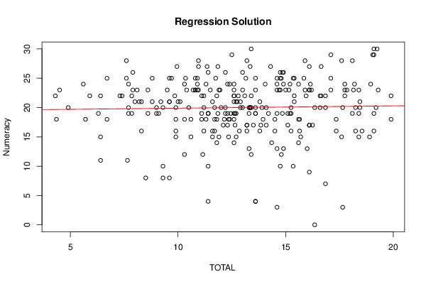
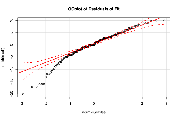
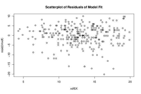
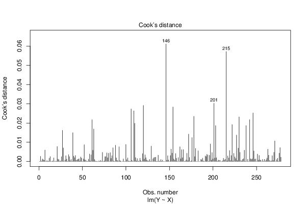
| Title produced by software | Simple Linear Regression | ||||||||||||||||||||||||||||||||||||||||||||||||||||||||||||||||||||||||||||||||||||||||||||||||||||||||||||||||||||||||||||||||||||||||||||||||||||||||||||||||||||||||
| Date of computation | Tue, 09 Dec 2014 12:47:37 +0000 | ||||||||||||||||||||||||||||||||||||||||||||||||||||||||||||||||||||||||||||||||||||||||||||||||||||||||||||||||||||||||||||||||||||||||||||||||||||||||||||||||||||||||
| Cite this page as follows | Statistical Computations at FreeStatistics.org, Office for Research Development and Education, URL https://freestatistics.org/blog/index.php?v=date/2014/Dec/09/t1418129283etcccvdw63vxrce.htm/, Retrieved Thu, 16 May 2024 11:35:50 +0000 | ||||||||||||||||||||||||||||||||||||||||||||||||||||||||||||||||||||||||||||||||||||||||||||||||||||||||||||||||||||||||||||||||||||||||||||||||||||||||||||||||||||||||
| Statistical Computations at FreeStatistics.org, Office for Research Development and Education, URL https://freestatistics.org/blog/index.php?pk=264536, Retrieved Thu, 16 May 2024 11:35:50 +0000 | |||||||||||||||||||||||||||||||||||||||||||||||||||||||||||||||||||||||||||||||||||||||||||||||||||||||||||||||||||||||||||||||||||||||||||||||||||||||||||||||||||||||||
| QR Codes: | |||||||||||||||||||||||||||||||||||||||||||||||||||||||||||||||||||||||||||||||||||||||||||||||||||||||||||||||||||||||||||||||||||||||||||||||||||||||||||||||||||||||||
|
| |||||||||||||||||||||||||||||||||||||||||||||||||||||||||||||||||||||||||||||||||||||||||||||||||||||||||||||||||||||||||||||||||||||||||||||||||||||||||||||||||||||||||
| Original text written by user: | |||||||||||||||||||||||||||||||||||||||||||||||||||||||||||||||||||||||||||||||||||||||||||||||||||||||||||||||||||||||||||||||||||||||||||||||||||||||||||||||||||||||||
| IsPrivate? | No (this computation is public) | ||||||||||||||||||||||||||||||||||||||||||||||||||||||||||||||||||||||||||||||||||||||||||||||||||||||||||||||||||||||||||||||||||||||||||||||||||||||||||||||||||||||||
| User-defined keywords | |||||||||||||||||||||||||||||||||||||||||||||||||||||||||||||||||||||||||||||||||||||||||||||||||||||||||||||||||||||||||||||||||||||||||||||||||||||||||||||||||||||||||
| Estimated Impact | 107 | ||||||||||||||||||||||||||||||||||||||||||||||||||||||||||||||||||||||||||||||||||||||||||||||||||||||||||||||||||||||||||||||||||||||||||||||||||||||||||||||||||||||||
Tree of Dependent Computations | |||||||||||||||||||||||||||||||||||||||||||||||||||||||||||||||||||||||||||||||||||||||||||||||||||||||||||||||||||||||||||||||||||||||||||||||||||||||||||||||||||||||||
| Family? (F = Feedback message, R = changed R code, M = changed R Module, P = changed Parameters, D = changed Data) | |||||||||||||||||||||||||||||||||||||||||||||||||||||||||||||||||||||||||||||||||||||||||||||||||||||||||||||||||||||||||||||||||||||||||||||||||||||||||||||||||||||||||
| - [Blocked Bootstrap Plot - Central Tendency] [] [2014-11-02 13:37:17] [cc401d1001c65f55a3dfc6f2420e9570] - RMPD [Simple Linear Regression] [] [2014-11-02 15:26:26] [cc401d1001c65f55a3dfc6f2420e9570] - RM [Simple Linear Regression] [] [2014-11-05 18:55:35] [e296091fd6311efcd9175c015e8e9c4e] - MPD [Simple Linear Regression] [] [2014-12-09 12:47:37] [72ee53c6f28232e74174360ca89644de] [Current] - PD [Simple Linear Regression] [] [2014-12-14 12:39:34] [36c866d94170840abc594fd3e7d5794f] - PD [Simple Linear Regression] [] [2014-12-14 12:50:11] [36c866d94170840abc594fd3e7d5794f] - D [Simple Linear Regression] [] [2014-12-14 12:55:18] [36c866d94170840abc594fd3e7d5794f] - D [Simple Linear Regression] [] [2014-12-14 12:59:02] [36c866d94170840abc594fd3e7d5794f] - D [Simple Linear Regression] [] [2014-12-14 13:02:17] [36c866d94170840abc594fd3e7d5794f] | |||||||||||||||||||||||||||||||||||||||||||||||||||||||||||||||||||||||||||||||||||||||||||||||||||||||||||||||||||||||||||||||||||||||||||||||||||||||||||||||||||||||||
| Feedback Forum | |||||||||||||||||||||||||||||||||||||||||||||||||||||||||||||||||||||||||||||||||||||||||||||||||||||||||||||||||||||||||||||||||||||||||||||||||||||||||||||||||||||||||
Post a new message | |||||||||||||||||||||||||||||||||||||||||||||||||||||||||||||||||||||||||||||||||||||||||||||||||||||||||||||||||||||||||||||||||||||||||||||||||||||||||||||||||||||||||
Dataset | |||||||||||||||||||||||||||||||||||||||||||||||||||||||||||||||||||||||||||||||||||||||||||||||||||||||||||||||||||||||||||||||||||||||||||||||||||||||||||||||||||||||||
| Dataseries X: | |||||||||||||||||||||||||||||||||||||||||||||||||||||||||||||||||||||||||||||||||||||||||||||||||||||||||||||||||||||||||||||||||||||||||||||||||||||||||||||||||||||||||
12.9 21 12.2 26 12.8 22 7.4 22 6.7 18 12.6 23 14.8 12 13.3 20 11.1 22 8.2 21 11.4 19 6.4 22 10.6 15 12 20 6.3 19 11.3 18 11.9 15 9.3 20 9.6 21 10 21 6.4 15 13.8 16 10.8 23 13.8 21 11.7 18 10.9 25 16.1 9 13.4 30 9.9 20 11.5 23 8.3 16 11.7 16 9 19 9.7 25 10.8 25 10.3 18 10.4 23 12.7 21 9.3 10 11.8 14 5.9 22 11.4 26 13 23 10.8 23 12.3 24 11.3 24 11.8 18 7.9 23 12.7 15 12.3 19 11.6 16 6.7 25 10.9 23 12.1 17 13.3 19 10.1 21 5.7 18 14.3 27 8 21 13.3 13 9.3 8 12.5 29 7.6 28 15.9 23 9.2 21 9.1 19 11.1 19 13 20 14.5 18 12.2 19 12.3 17 11.4 19 8.8 25 14.6 19 12.6 22 13 26 12.6 14 13.2 28 9.9 16 7.7 24 10.5 20 13.4 12 10.9 24 4.3 22 10.3 12 11.8 22 11.2 20 11.4 10 8.6 23 13.2 17 12.6 22 5.6 24 9.9 18 8.8 21 7.7 20 9 20 7.3 22 11.4 19 13.6 20 7.9 26 10.7 23 10.3 24 8.3 21 9.6 21 14.2 19 8.5 8 13.5 17 4.9 20 6.4 11 9.6 8 11.6 15 11.1 18 4.35 18 12.7 19 18.1 19 17.85 23 16.6 22 12.6 21 17.1 25 19.1 30 16.1 17 13.35 27 18.4 23 14.7 23 10.6 18 12.6 18 16.2 23 13.6 19 18.9 15 14.1 20 14.5 16 16.15 24 14.75 25 14.8 25 12.45 19 12.65 19 17.35 16 8.6 19 18.4 19 16.1 23 11.6 21 17.75 22 15.25 19 17.65 20 16.35 20 17.65 3 13.6 23 14.35 14 14.75 23 18.25 20 9.9 15 16 13 18.25 16 16.85 7 14.6 24 13.85 17 18.95 24 15.6 24 14.85 19 11.75 25 18.45 20 15.9 28 17.1 23 16.1 27 19.9 18 10.95 28 18.45 21 15.1 19 15 23 11.35 27 15.95 22 18.1 28 14.6 25 15.4 21 15.4 22 17.6 28 13.35 20 19.1 29 15.35 25 7.6 25 13.4 20 13.9 20 19.1 16 15.25 20 12.9 20 16.1 23 17.35 18 13.15 25 12.15 18 12.6 19 10.35 25 15.4 25 9.6 25 18.2 24 13.6 19 14.85 26 14.75 10 14.1 17 14.9 13 16.25 17 19.25 30 13.6 25 13.6 4 15.65 16 12.75 21 14.6 23 9.85 22 12.65 17 19.2 20 16.6 20 11.2 22 15.25 16 11.9 23 13.2 16 16.35 0 12.4 18 15.85 25 18.15 23 11.15 12 15.65 18 17.75 24 7.65 11 12.35 18 15.6 14 19.3 23 15.2 24 17.1 29 15.6 18 18.4 15 19.05 29 18.55 16 19.1 19 13.1 22 12.85 16 9.5 23 4.5 23 11.85 19 13.6 4 11.7 20 12.4 24 13.35 20 11.4 4 14.9 24 19.9 22 11.2 16 14.6 3 17.6 15 14.05 24 16.1 17 13.35 20 11.85 27 11.95 23 14.75 26 15.15 23 13.2 17 16.85 20 7.85 22 7.7 19 12.6 24 7.85 19 10.95 23 12.35 15 9.95 27 14.9 26 16.65 22 13.4 22 13.95 18 15.7 15 16.85 22 10.95 27 15.35 10 12.2 20 15.1 17 17.75 23 15.2 19 14.6 13 16.65 27 8.1 23 | |||||||||||||||||||||||||||||||||||||||||||||||||||||||||||||||||||||||||||||||||||||||||||||||||||||||||||||||||||||||||||||||||||||||||||||||||||||||||||||||||||||||||
Tables (Output of Computation) | |||||||||||||||||||||||||||||||||||||||||||||||||||||||||||||||||||||||||||||||||||||||||||||||||||||||||||||||||||||||||||||||||||||||||||||||||||||||||||||||||||||||||
| |||||||||||||||||||||||||||||||||||||||||||||||||||||||||||||||||||||||||||||||||||||||||||||||||||||||||||||||||||||||||||||||||||||||||||||||||||||||||||||||||||||||||
Figures (Output of Computation) | |||||||||||||||||||||||||||||||||||||||||||||||||||||||||||||||||||||||||||||||||||||||||||||||||||||||||||||||||||||||||||||||||||||||||||||||||||||||||||||||||||||||||
Input Parameters & R Code | |||||||||||||||||||||||||||||||||||||||||||||||||||||||||||||||||||||||||||||||||||||||||||||||||||||||||||||||||||||||||||||||||||||||||||||||||||||||||||||||||||||||||
| Parameters (Session): | |||||||||||||||||||||||||||||||||||||||||||||||||||||||||||||||||||||||||||||||||||||||||||||||||||||||||||||||||||||||||||||||||||||||||||||||||||||||||||||||||||||||||
| par1 = 1 ; par2 = 2 ; par3 = Exact Pearson Chi-Squared by Simulation ; | |||||||||||||||||||||||||||||||||||||||||||||||||||||||||||||||||||||||||||||||||||||||||||||||||||||||||||||||||||||||||||||||||||||||||||||||||||||||||||||||||||||||||
| Parameters (R input): | |||||||||||||||||||||||||||||||||||||||||||||||||||||||||||||||||||||||||||||||||||||||||||||||||||||||||||||||||||||||||||||||||||||||||||||||||||||||||||||||||||||||||
| par1 = 2 ; par2 = 1 ; par3 = TRUE ; | |||||||||||||||||||||||||||||||||||||||||||||||||||||||||||||||||||||||||||||||||||||||||||||||||||||||||||||||||||||||||||||||||||||||||||||||||||||||||||||||||||||||||
| R code (references can be found in the software module): | |||||||||||||||||||||||||||||||||||||||||||||||||||||||||||||||||||||||||||||||||||||||||||||||||||||||||||||||||||||||||||||||||||||||||||||||||||||||||||||||||||||||||
cat1 <- as.numeric(par1) | |||||||||||||||||||||||||||||||||||||||||||||||||||||||||||||||||||||||||||||||||||||||||||||||||||||||||||||||||||||||||||||||||||||||||||||||||||||||||||||||||||||||||