Free Statistics
of Irreproducible Research!
Description of Statistical Computation | |||||||||||||||||||||
|---|---|---|---|---|---|---|---|---|---|---|---|---|---|---|---|---|---|---|---|---|---|
| Author's title | |||||||||||||||||||||
| Author | *The author of this computation has been verified* | ||||||||||||||||||||
| R Software Module | rwasp_sdplot.wasp | ||||||||||||||||||||
| Title produced by software | Standard Deviation Plot | ||||||||||||||||||||
| Date of computation | Tue, 09 Dec 2014 16:06:38 +0000 | ||||||||||||||||||||
| Cite this page as follows | Statistical Computations at FreeStatistics.org, Office for Research Development and Education, URL https://freestatistics.org/blog/index.php?v=date/2014/Dec/09/t1418141212bxacpj4j46v4eof.htm/, Retrieved Thu, 16 May 2024 10:58:23 +0000 | ||||||||||||||||||||
| Statistical Computations at FreeStatistics.org, Office for Research Development and Education, URL https://freestatistics.org/blog/index.php?pk=264728, Retrieved Thu, 16 May 2024 10:58:23 +0000 | |||||||||||||||||||||
| QR Codes: | |||||||||||||||||||||
|
| |||||||||||||||||||||
| Original text written by user: | |||||||||||||||||||||
| IsPrivate? | No (this computation is public) | ||||||||||||||||||||
| User-defined keywords | |||||||||||||||||||||
| Estimated Impact | 69 | ||||||||||||||||||||
Tree of Dependent Computations | |||||||||||||||||||||
| Family? (F = Feedback message, R = changed R code, M = changed R Module, P = changed Parameters, D = changed Data) | |||||||||||||||||||||
| - [Mean versus Median] [] [2014-12-08 16:25:59] [78252ca1523d3477f114bddbfa59edb4] - RMP [Standard Deviation Plot] [] [2014-12-09 16:06:38] [54099b55f731ed0aca9a713a2b2a06c3] [Current] | |||||||||||||||||||||
| Feedback Forum | |||||||||||||||||||||
Post a new message | |||||||||||||||||||||
Dataset | |||||||||||||||||||||
| Dataseries X: | |||||||||||||||||||||
1894,00 1757,00 3582,00 5321,00 5561,00 5907,00 4944,00 4966,00 3258,00 1964,00 1743,00 1262,00 2086,00 1793,00 3548,00 5672,00 6084,00 4914,00 4990,00 5139,00 3218,00 2179,00 2238,00 1442,00 2205,00 2025,00 3531,00 4977,00 7998,00 4880,00 5231,00 5202,00 3303,00 2683,00 2202,00 1376,00 2422,00 1997,00 3163,00 5964,00 5657,00 6415,00 6208,00 4500,00 2939,00 2702,00 2090,00 1504,00 2549,00 1931,00 3013,00 6204,00 5788,00 5611,00 5594,00 4647,00 3490,00 2487,00 1992,00 1507,00 2306,00 2002,00 3075,00 5331,00 5589,00 5813,00 4876,00 4665,00 3601,00 2192,00 2111,00 1580,00 2288,00 1993,00 3228,00 5000,00 5480,00 5770,00 4962,00 4685,00 3607,00 2222,00 2467,00 1594,00 2228,00 1910,00 3157,00 4809,00 6249,00 4607,00 4975,00 4784,00 3028,00 2461,00 2218,00 1351,00 2070,00 1887,00 3024,00 4596,00 6398,00 4459,00 5382,00 4359,00 2687,00 2249,00 2154,00 1169,00 2429,00 1762,00 2846,00 5627,00 5749,00 4502,00 5720,00 4403,00 2867,00 2635,00 2059,00 1511,00 2359,00 1741,00 2917,00 6249,00 5760,00 6250,00 5134,00 4831,00 3695,00 2462,00 2146,00 1579,00 | |||||||||||||||||||||
Tables (Output of Computation) | |||||||||||||||||||||
| |||||||||||||||||||||
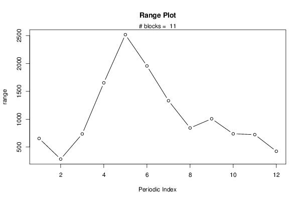
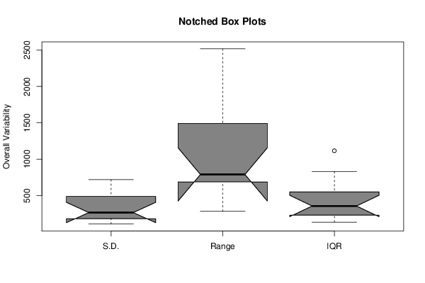
Figures (Output of Computation) | |||||||||||||||||||||
Input Parameters & R Code | |||||||||||||||||||||
| Parameters (Session): | |||||||||||||||||||||
| par1 = 12 ; | |||||||||||||||||||||
| Parameters (R input): | |||||||||||||||||||||
| par1 = 12 ; | |||||||||||||||||||||
| R code (references can be found in the software module): | |||||||||||||||||||||
par1 <- '12' | |||||||||||||||||||||