Free Statistics
of Irreproducible Research!
Description of Statistical Computation | |||||||||||||||||||||||||||||||||||||||||||||
|---|---|---|---|---|---|---|---|---|---|---|---|---|---|---|---|---|---|---|---|---|---|---|---|---|---|---|---|---|---|---|---|---|---|---|---|---|---|---|---|---|---|---|---|---|---|
| Author's title | |||||||||||||||||||||||||||||||||||||||||||||
| Author | *The author of this computation has been verified* | ||||||||||||||||||||||||||||||||||||||||||||
| R Software Module | rwasp_bidensity.wasp | ||||||||||||||||||||||||||||||||||||||||||||
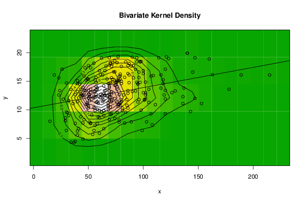
| Title produced by software | Bivariate Kernel Density Estimation | ||||||||||||||||||||||||||||||||||||||||||||
| Date of computation | Tue, 09 Dec 2014 16:25:19 +0000 | ||||||||||||||||||||||||||||||||||||||||||||
| Cite this page as follows | Statistical Computations at FreeStatistics.org, Office for Research Development and Education, URL https://freestatistics.org/blog/index.php?v=date/2014/Dec/09/t1418142332vow0h1t93ygf2mf.htm/, Retrieved Thu, 16 May 2024 14:30:01 +0000 | ||||||||||||||||||||||||||||||||||||||||||||
| Statistical Computations at FreeStatistics.org, Office for Research Development and Education, URL https://freestatistics.org/blog/index.php?pk=264743, Retrieved Thu, 16 May 2024 14:30:01 +0000 | |||||||||||||||||||||||||||||||||||||||||||||
| QR Codes: | |||||||||||||||||||||||||||||||||||||||||||||
|
| |||||||||||||||||||||||||||||||||||||||||||||
| Original text written by user: | |||||||||||||||||||||||||||||||||||||||||||||
| IsPrivate? | No (this computation is public) | ||||||||||||||||||||||||||||||||||||||||||||
| User-defined keywords | |||||||||||||||||||||||||||||||||||||||||||||
| Estimated Impact | 87 | ||||||||||||||||||||||||||||||||||||||||||||
Tree of Dependent Computations | |||||||||||||||||||||||||||||||||||||||||||||
| Family? (F = Feedback message, R = changed R code, M = changed R Module, P = changed Parameters, D = changed Data) | |||||||||||||||||||||||||||||||||||||||||||||
| - [Pearson Correlation] [] [2014-12-09 16:07:49] [fa1b8827d7de91b8b87087311d3d9fa1] - RMPD [Bivariate Kernel Density Estimation] [] [2014-12-09 16:19:40] [7b949ef3605c038fc6e10efeab34f433] - R D [Bivariate Kernel Density Estimation] [] [2014-12-09 16:25:19] [aa823bdb4d51626f3fbc68989a46faf3] [Current] | |||||||||||||||||||||||||||||||||||||||||||||
| Feedback Forum | |||||||||||||||||||||||||||||||||||||||||||||
Post a new message | |||||||||||||||||||||||||||||||||||||||||||||
Dataset | |||||||||||||||||||||||||||||||||||||||||||||
| Dataseries X: | |||||||||||||||||||||||||||||||||||||||||||||
86 70 71 108 64 119 97 129 153 78 80 99 68 147 40 57 120 71 84 68 55 137 79 116 101 111 189 66 81 63 69 71 64 143 85 86 55 69 120 96 60 95 100 68 57 105 85 103 57 51 69 41 49 50 93 58 54 74 15 69 107 65 58 107 70 53 136 126 95 69 136 58 59 118 82 102 65 90 64 83 70 50 77 37 81 101 79 71 60 55 44 40 56 43 45 32 56 40 34 89 50 56 46 76 64 74 57 45 30 62 51 36 34 61 70 69 145 23 120 147 215 24 84 30 77 46 61 178 160 57 42 163 75 94 45 78 47 29 97 116 32 50 118 66 86 89 76 75 57 72 60 109 76 65 40 58 123 71 102 80 97 46 93 19 140 78 98 40 80 76 79 87 95 49 49 80 86 69 79 52 120 69 94 72 43 87 52 71 61 51 50 67 30 70 52 75 87 69 72 79 121 43 58 57 50 69 64 38 90 96 49 56 102 40 100 67 78 55 59 96 86 38 43 23 77 48 26 91 94 62 74 114 52 64 31 38 27 105 64 62 65 58 76 140 68 80 71 76 63 46 53 74 70 78 56 100 51 52 102 78 78 55 98 76 73 47 45 83 60 48 50 56 77 91 76 68 74 29 | |||||||||||||||||||||||||||||||||||||||||||||
| Dataseries Y: | |||||||||||||||||||||||||||||||||||||||||||||
12.9 12.2 12.8 7.4 6.7 12.6 14.8 13.3 11.1 8.2 11.4 6.4 10.6 12 6.3 11.3 11.9 9.3 9.6 10 6.4 13.8 10.8 13.8 11.7 10.9 16.1 13.4 9.9 11.5 8.3 11.7 9 9.7 10.8 10.3 10.4 12.7 9.3 11.8 5.9 11.4 13 10.8 12.3 11.3 11.8 7.9 12.7 12.3 11.6 6.7 10.9 12.1 13.3 10.1 5.7 14.3 8 13.3 9.3 12.5 7.6 15.9 9.2 9.1 11.1 13 14.5 12.2 12.3 11.4 8.8 14.6 12.6 13 12.6 13.2 9.9 7.7 10.5 13.4 10.9 4.3 10.3 11.8 11.2 11.4 8.6 13.2 12.6 5.6 9.9 8.8 7.7 9 7.3 11.4 13.6 7.9 10.7 10.3 8.3 9.6 14.2 8.5 13.5 4.9 6.4 9.6 11.6 11.1 4.35 12.7 18.1 17.85 16.6 12.6 17.1 19.1 16.1 13.35 18.4 14.7 10.6 12.6 16.2 13.6 18.9 14.1 14.5 16.15 14.75 14.8 12.45 12.65 17.35 8.6 18.4 16.1 11.6 17.75 15.25 17.65 16.35 17.65 13.6 14.35 14.75 18.25 9.9 16 18.25 16.85 14.6 13.85 18.95 15.6 14.85 11.75 18.45 15.9 17.1 16.1 19.9 10.95 18.45 15.1 15 11.35 15.95 18.1 14.6 15.4 15.4 17.6 13.35 19.1 15.35 7.6 13.4 13.9 19.1 15.25 12.9 16.1 17.35 13.15 12.15 12.6 10.35 15.4 9.6 18.2 13.6 14.85 14.75 14.1 14.9 16.25 19.25 13.6 13.6 15.65 12.75 14.6 9.85 12.65 19.2 16.6 11.2 15.25 11.9 13.2 16.35 12.4 15.85 18.15 11.15 15.65 17.75 7.65 12.35 15.6 19.3 15.2 17.1 15.6 18.4 19.05 18.55 19.1 13.1 12.85 9.5 4.5 11.85 13.6 11.7 12.4 13.35 11.4 14.9 19.9 11.2 14.6 17.6 14.05 16.1 13.35 11.85 11.95 14.75 15.15 13.2 16.85 7.85 7.7 12.6 7.85 10.95 12.35 9.95 14.9 16.65 13.4 13.95 15.7 16.85 10.95 15.35 12.2 15.1 17.75 15.2 14.6 16.65 8.1 | |||||||||||||||||||||||||||||||||||||||||||||
Tables (Output of Computation) | |||||||||||||||||||||||||||||||||||||||||||||
| |||||||||||||||||||||||||||||||||||||||||||||
Figures (Output of Computation) | |||||||||||||||||||||||||||||||||||||||||||||
Input Parameters & R Code | |||||||||||||||||||||||||||||||||||||||||||||
| Parameters (Session): | |||||||||||||||||||||||||||||||||||||||||||||
| par1 = grey ; | |||||||||||||||||||||||||||||||||||||||||||||
| Parameters (R input): | |||||||||||||||||||||||||||||||||||||||||||||
| par1 = 20 ; par2 = 5 ; par3 = 0 ; par4 = 0 ; par5 = 0 ; par6 = Y ; par7 = Y ; par8 = terrain.colors ; | |||||||||||||||||||||||||||||||||||||||||||||
| R code (references can be found in the software module): | |||||||||||||||||||||||||||||||||||||||||||||
par8 <- 'terrain.colors' | |||||||||||||||||||||||||||||||||||||||||||||