Free Statistics
of Irreproducible Research!
Description of Statistical Computation | |||||||||||||||||||||||||||||||||||||||||||||
|---|---|---|---|---|---|---|---|---|---|---|---|---|---|---|---|---|---|---|---|---|---|---|---|---|---|---|---|---|---|---|---|---|---|---|---|---|---|---|---|---|---|---|---|---|---|
| Author's title | |||||||||||||||||||||||||||||||||||||||||||||
| Author | *The author of this computation has been verified* | ||||||||||||||||||||||||||||||||||||||||||||
| R Software Module | rwasp_bidensity.wasp | ||||||||||||||||||||||||||||||||||||||||||||
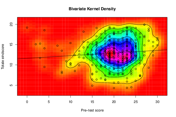
| Title produced by software | Bivariate Kernel Density Estimation | ||||||||||||||||||||||||||||||||||||||||||||
| Date of computation | Tue, 09 Dec 2014 18:56:45 +0000 | ||||||||||||||||||||||||||||||||||||||||||||
| Cite this page as follows | Statistical Computations at FreeStatistics.org, Office for Research Development and Education, URL https://freestatistics.org/blog/index.php?v=date/2014/Dec/09/t1418151716qlzngc0znf8cj6g.htm/, Retrieved Thu, 16 May 2024 10:42:22 +0000 | ||||||||||||||||||||||||||||||||||||||||||||
| Statistical Computations at FreeStatistics.org, Office for Research Development and Education, URL https://freestatistics.org/blog/index.php?pk=264813, Retrieved Thu, 16 May 2024 10:42:22 +0000 | |||||||||||||||||||||||||||||||||||||||||||||
| QR Codes: | |||||||||||||||||||||||||||||||||||||||||||||
|
| |||||||||||||||||||||||||||||||||||||||||||||
| Original text written by user: | |||||||||||||||||||||||||||||||||||||||||||||
| IsPrivate? | No (this computation is public) | ||||||||||||||||||||||||||||||||||||||||||||
| User-defined keywords | |||||||||||||||||||||||||||||||||||||||||||||
| Estimated Impact | 105 | ||||||||||||||||||||||||||||||||||||||||||||
Tree of Dependent Computations | |||||||||||||||||||||||||||||||||||||||||||||
| Family? (F = Feedback message, R = changed R code, M = changed R Module, P = changed Parameters, D = changed Data) | |||||||||||||||||||||||||||||||||||||||||||||
| - [Percentiles] [Intrinsic Motivat...] [2010-10-12 12:10:58] [b98453cac15ba1066b407e146608df68] - RMPD [Kernel Density Estimation] [] [2011-10-18 22:42:23] [b98453cac15ba1066b407e146608df68] - RMPD [Percentiles] [] [2011-10-18 22:46:45] [b98453cac15ba1066b407e146608df68] - RMPD [Notched Boxplots] [] [2011-10-18 22:58:56] [b98453cac15ba1066b407e146608df68] - RM D [Back to Back Histogram] [] [2011-10-18 23:05:48] [b98453cac15ba1066b407e146608df68] - RMPD [Back to Back Histogram] [] [2014-12-09 17:55:01] [ea990983fba95a758c0bb6d29c9aee24] - RMPD [Bivariate Kernel Density Estimation] [] [2014-12-09 18:56:45] [6260c34aa94cecca073345f42e0d4b5d] [Current] | |||||||||||||||||||||||||||||||||||||||||||||
| Feedback Forum | |||||||||||||||||||||||||||||||||||||||||||||
Post a new message | |||||||||||||||||||||||||||||||||||||||||||||
Dataset | |||||||||||||||||||||||||||||||||||||||||||||
| Dataseries X: | |||||||||||||||||||||||||||||||||||||||||||||
21 26 22 22 18 23 12 20 22 21 19 22 15 20 19 18 15 20 21 21 15 16 23 21 18 25 9 30 20 23 16 16 19 25 25 18 23 21 10 14 22 26 23 23 24 24 18 23 15 19 16 25 23 17 19 21 18 27 21 13 8 29 28 23 21 19 19 20 18 19 17 19 25 19 22 23 26 14 28 16 24 20 12 24 22 12 22 20 10 23 17 22 24 18 21 20 20 22 19 20 26 23 24 21 21 19 8 17 20 11 8 15 18 18 19 19 23 22 21 25 30 17 27 23 23 18 18 23 19 15 20 16 24 25 25 19 19 16 19 19 23 21 22 19 20 20 3 23 14 23 20 15 13 16 7 24 17 24 24 19 25 20 28 23 27 18 28 21 19 23 27 22 28 25 21 22 28 20 29 25 25 20 20 16 20 20 23 18 25 18 19 25 25 25 24 19 26 10 17 13 17 30 25 4 16 21 23 22 17 20 20 22 16 23 16 0 18 25 23 12 18 24 11 18 14 23 24 29 18 15 29 16 19 22 16 23 23 19 4 20 24 20 4 24 22 16 3 15 24 17 20 27 23 26 23 17 20 22 19 24 19 23 15 27 26 22 22 18 15 22 27 10 20 17 23 19 13 27 23 16 25 2 26 20 23 22 24 | |||||||||||||||||||||||||||||||||||||||||||||
| Dataseries Y: | |||||||||||||||||||||||||||||||||||||||||||||
12.9 7.4 12.2 12.8 7.4 6.7 12.6 14.8 13.3 11.1 8.2 11.4 6.4 10.6 12.0 6.3 11.3 11.9 9.3 9.6 10.0 6.4 13.8 10.8 13.8 11.7 10.9 16.1 13.4 9.9 11.5 8.3 11.7 6.1 9.0 9.7 10.8 10.3 10.4 12.7 9.3 11.8 5.9 11.4 13.0 10.8 12.3 11.3 11.8 7.9 12.7 12.3 11.6 6.7 10.9 12.1 13.3 10.1 5.7 14.3 8.0 13.3 9.3 12.5 7.6 15.9 9.2 9.1 11.1 13.0 14.5 12.2 12.3 11.4 8.8 14.6 7.3 12.6 NA 13.0 12.6 13.2 9.9 7.7 10.5 13.4 10.9 4.3 10.3 11.8 11.2 11.4 8.6 13.2 12.6 5.6 9.9 8.8 7.7 9.0 7.3 11.4 13.6 7.9 10.7 10.3 8.3 9.6 14.2 8.5 13.5 4.9 6.4 9.6 11.6 11.1 4.35 12.7 18.1 17.85 16.6 12.6 17.1 19.1 16.1 13.35 18.4 14.7 10.6 12.6 16.2 13.6 18.9 14.1 14.5 16.15 14.75 14.8 12.45 12.65 17.35 8.6 18.4 16.1 11.6 17.75 15.25 17.65 15.6 16.35 17.65 13.6 11.7 14.35 14.75 18.25 9.9 16 18.25 16.85 14.6 13.85 18.95 15.6 14.85 11.75 18.45 15.9 17.1 16.1 19.9 10.95 18.45 15.1 15 11.35 15.95 18.1 14.6 15.4 15.4 17.6 13.35 19.1 15.35 7.6 13.4 13.9 19.1 15.25 12.9 16.1 17.35 13.15 12.15 12.6 10.35 15.4 9.6 18.2 13.6 14.85 14.75 14.1 14.9 16.25 19.25 13.6 13.6 15.65 12.75 14.6 9.85 12.65 11.9 19.2 16.6 11.2 15.25 11.9 13.2 16.35 12.4 15.85 14.35 18.15 11.15 15.65 17.75 7.65 12.35 15.6 19.3 15.2 17.1 15.6 18.4 19.05 18.55 19.1 13.1 12.85 9.5 4.5 11.85 13.6 11.7 12.4 13.35 11.4 14.9 19.9 17.75 11.2 14.6 17.6 14.05 16.1 13.35 11.85 11.95 14.75 15.15 13.2 16.85 7.85 7.7 12.6 7.85 10.95 12.35 9.95 14.9 16.65 13.4 13.95 15.7 16.85 10.95 15.35 12.2 15.1 17.75 15.2 14.6 16.65 8.1 | |||||||||||||||||||||||||||||||||||||||||||||
Tables (Output of Computation) | |||||||||||||||||||||||||||||||||||||||||||||
| |||||||||||||||||||||||||||||||||||||||||||||
Figures (Output of Computation) | |||||||||||||||||||||||||||||||||||||||||||||
Input Parameters & R Code | |||||||||||||||||||||||||||||||||||||||||||||
| Parameters (Session): | |||||||||||||||||||||||||||||||||||||||||||||
| Parameters (R input): | |||||||||||||||||||||||||||||||||||||||||||||
| par1 = 50 ; par2 = 50 ; par3 = 0 ; par4 = 0 ; par5 = 0 ; par6 = Y ; par7 = Y ; par8 = rainbow ; | |||||||||||||||||||||||||||||||||||||||||||||
| R code (references can be found in the software module): | |||||||||||||||||||||||||||||||||||||||||||||
par8 <- 'rainbow' | |||||||||||||||||||||||||||||||||||||||||||||