Repository of Reproducible Computations

Free Statistics

of Irreproducible Research!

Author's title

Author

*The author of this computation has been verified*

R Software Module

rwasp_pairs.wasp

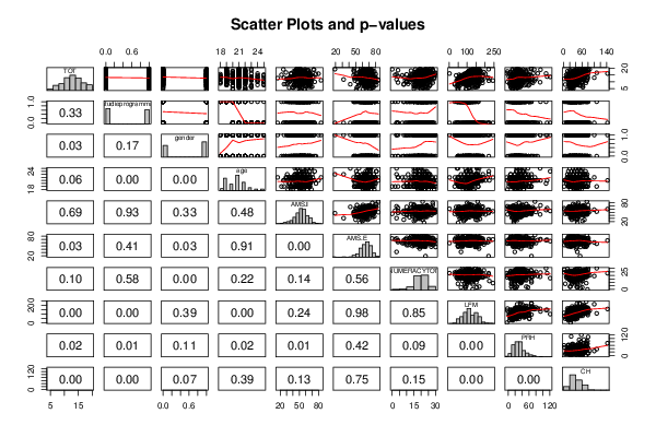
Title produced by software

Kendall tau Correlation Matrix

Date of computation

Thu, 11 Dec 2014 10:27:55 +0000

Cite this page as follows

Statistical Computations at FreeStatistics.org, Office for Research Development and Education, URL https://freestatistics.org/blog/index.php?v=date/2014/Dec/11/t14182937214a0ec2n1smjxbds.htm/, Retrieved Thu, 16 May 2024 15:10:17 +0000

Statistical Computations at FreeStatistics.org, Office for Research Development and Education, URL https://freestatistics.org/blog/index.php?pk=265680, Retrieved Thu, 16 May 2024 15:10:17 +0000

QR Codes:

Paste this QR Code to cite your computation.

Original text written by user:

IsPrivate?

No (this computation is public)

User-defined keywords

Estimated Impact

110

Family? (F = Feedback message, R = changed R code, M = changed R Module, P = changed Parameters, D = changed Data)

-       [Kendall tau Correlation Matrix] [pearson correlati...] [2014-12-11 10:27:55] [d71ad52285d92a63edfc83f9fb1da7a1] [Current]

Feedback Forum

Post a new message

Dataseries X:

Download CSV

Histogram

Boxplots

12.9 0 0 21 26 50 21 149 18 68
7.4 0 0 23 51 68 26 152 7 55
12.2 0 1 22 57 62 22 139 31 39
12.8 0 0 21 37 54 22 148 39 32
7.4 0 1 21 67 71 18 158 46 62
6.7 0 1 21 43 54 23 128 31 33
12.6 0 1 21 52 65 12 224 67 52
14.8 0 0 21 52 73 20 159 35 62
13.3 0 1 23 43 52 22 105 52 77
11.1 0 1 22 84 84 21 159 77 76
8.2 0 1 25 67 42 19 167 37 41
11.4 0 1 21 49 66 22 165 32 48
6.4 0 1 23 70 65 15 159 36 63
10.6 0 1 22 52 78 20 119 38 30
12 0 0 21 58 73 19 176 69 78
6.3 0 0 21 68 75 18 54 21 19
11.3 1 0 25 62 72 15 91 26 31
11.9 0 1 21 43 66 20 163 54 66
9.3 0 0 21 56 70 21 124 36 35
9.6 1 1 20 56 61 21 137 42 42
10 0 0 24 74 81 15 121 23 45
6.4 0 1 23 65 71 16 153 34 21
13.8 0 1 21 63 69 23 148 112 25
10.8 0 0 24 58 71 21 221 35 44
13.8 0 1 23 57 72 18 188 47 69
11.7 0 1 21 63 68 25 149 47 54
10.9 0 1 22 53 70 9 244 37 74
16.1 1 1 20 57 68 30 148 109 80
13.4 1 0 18 51 61 20 92 24 42
9.9 0 1 21 64 67 23 150 20 61
11.5 0 0 22 53 76 16 153 22 41
8.3 0 0 22 29 70 16 94 23 46
11.7 0 0 21 54 60 19 156 32 39
6.1 0 1 23 51 77 25 146 7 63
9 0 1 21 58 72 25 132 30 34
9.7 0 1 25 43 69 18 161 92 51
10.8 0 1 22 51 71 23 105 43 42
10.3 0 1 22 53 62 21 97 55 31
10.4 0 0 20 54 70 10 151 16 39
12.7 1 1 21 56 64 14 131 49 20
9.3 0 1 21 61 58 22 166 71 49
11.8 0 0 21 47 76 26 157 43 53
5.9 0 1 22 39 52 23 111 29 31
11.4 0 1 21 48 59 23 145 56 39
13 0 1 24 50 68 24 162 46 54
10.8 0 1 22 35 76 24 163 19 49
12.3 1 1 22 30 65 18 59 23 34
11.3 0 0 21 68 67 23 187 59 46
11.8 0 1 22 49 59 15 109 30 55
7.9 1 1 19 61 69 19 90 61 42
12.7 0 0 22 67 76 16 105 7 50
12.3 1 1 23 47 63 25 83 38 13
11.6 1 1 20 56 75 23 116 32 37
6.7 1 1 20 50 63 17 42 16 25
10.9 0 1 23 43 60 19 148 19 30
12.1 1 1 20 67 73 21 155 22 28
13.3 0 1 23 62 63 18 125 48 45
10.1 0 1 21 57 70 27 116 23 35
5.7 1 0 22 41 75 21 128 26 28
14.3 0 1 21 54 66 13 138 33 41
8 1 0 21 45 63 8 49 9 6
13.3 1 1 19 48 63 29 96 24 45
9.3 0 1 22 61 64 28 164 34 73
12.5 0 0 21 56 70 23 162 48 17
7.6 0 0 21 41 75 21 99 18 40
15.9 0 1 21 43 61 19 202 43 64
9.2 0 0 21 53 60 19 186 33 37
9.1 1 1 21 44 62 20 66 28 25
11.1 0 0 21 66 73 18 183 71 65
13 0 1 22 58 61 19 214 26 100
14.5 0 1 22 46 66 17 188 67 28
12.2 1 0 18 37 64 19 104 34 35
12.3 0 0 21 51 59 25 177 80 56
11.4 0 0 23 51 64 19 126 29 29
8.8 1 0 19 56 60 22 76 16 43
14.6 1 1 19 66 56 23 99 59 59
7.3 0 1 23 45 66 26 157 58 52
12.6 0 0 21 37 78 14 139 32 50
NA 0 1 21 59 53 28 78 47 3
13 0 0 21 42 67 16 162 43 59
12.6 1 1 21 38 59 24 108 38 27
13.2 0 0 20 66 66 20 159 29 61
9.9 1 0 19 34 68 12 74 36 28
7.7 0 1 21 53 71 24 110 32 51
10.5 1 0 19 49 66 22 96 35 35
13.4 1 0 19 55 73 12 116 21 29
10.9 1 0 19 49 72 22 87 29 48
4.3 1 1 20 59 71 20 97 12 25
10.3 1 0 19 40 59 10 127 37 44
11.8 1 1 19 58 64 23 106 37 64
11.2 1 1 19 60 66 17 80 47 32
11.4 1 0 20 63 78 22 74 51 20
8.6 1 0 19 56 68 24 91 32 28
13.2 1 0 18 54 73 18 133 21 34
12.6 1 1 19 52 62 21 74 13 31
5.6 1 1 21 34 65 20 114 14 26
9.9 1 1 18 69 68 20 140 -2 58
8.8 1 0 18 32 65 22 95 20 23
7.7 1 1 19 48 60 19 98 24 21
9 1 0 21 67 71 20 121 11 21
7.3 1 1 20 58 65 26 126 23 33
11.4 1 1 24 57 68 23 98 24 16
13.6 1 1 22 42 64 24 95 14 20
7.9 1 1 21 64 74 21 110 52 37
10.7 1 1 21 58 69 21 70 15 35
10.3 1 0 19 66 76 19 102 23 33
8.3 1 1 19 26 68 8 86 19 27
9.6 1 1 20 61 72 17 130 35 41
14.2 1 1 18 52 67 20 96 24 40
8.5 1 0 19 51 63 11 102 39 35
13.5 1 0 19 55 59 8 100 29 28
4.9 1 0 20 50 73 15 94 13 32
6.4 1 0 21 60 66 18 52 8 22
9.6 1 0 18 56 62 18 98 18 44
11.6 1 0 19 63 69 19 118 24 27
11.1 1 1 19 61 66 19 99 19 17
4.35 0 1 22 52 51 23 48 23 12
12.7 0 1 22 16 56 22 50 16 45
18.1 0 1 22 46 67 21 150 33 37
17.85 0 1 20 56 69 25 154 32 37
16.6 1 0 19 52 57 30 109 37 108
12.6 1 1 20 55 56 17 68 14 10
17.1 0 1 22 50 55 27 194 52 68
19.1 0 0 21 59 63 23 158 75 72
16.1 0 1 21 60 67 23 159 72 143
13.35 0 0 21 52 65 18 67 15 9
18.4 0 0 21 44 47 18 147 29 55
14.7 0 1 21 67 76 23 39 13 17
10.6 0 1 21 52 64 19 100 40 37
12.6 0 1 21 55 68 15 111 19 27
16.2 0 1 22 37 64 20 138 24 37
13.6 0 1 24 54 65 16 101 121 58
18.9 1 1 21 72 71 24 131 93 66
14.1 0 1 22 51 63 25 101 36 21
14.5 0 1 20 48 60 25 114 23 19
16.15 0 0 21 60 68 19 165 85 78
14.75 0 1 24 50 72 19 114 41 35
14.8 0 1 25 63 70 16 111 46 48
12.45 0 1 22 33 61 19 75 18 27
12.65 0 1 21 67 61 19 82 35 43
17.35 0 1 21 46 62 23 121 17 30
8.6 0 1 22 54 71 21 32 4 25
18.4 0 0 23 59 71 22 150 28 69
16.1 0 1 24 61 51 19 117 44 72
11.6 1 1 20 33 56 20 71 10 23
17.75 0 1 22 47 70 20 165 38 13
15.25 0 1 25 69 73 3 154 57 61
17.65 0 1 22 52 76 23 126 23 43
15.6 0 0 22 55 59 14 138 26 22
16.35 0 0 21 55 68 23 149 36 51
17.65 0 0 21 41 48 20 145 22 67
13.6 0 1 21 73 52 15 120 40 36
11.7 0 0 22 51 59 13 138 18 21
14.35 0 0 22 52 60 16 109 31 44
14.75 0 0 22 50 59 7 132 11 45
18.25 0 1 21 51 57 24 172 38 34
9.9 0 0 22 60 79 17 169 24 36
16 0 1 23 56 60 24 114 37 72
18.25 0 1 21 56 60 24 156 37 39
16.85 0 0 21 29 59 19 172 22 43
14.6 1 1 21 66 62 25 68 15 25
13.85 1 1 19 66 59 20 89 2 56
18.95 0 1 21 73 61 28 167 43 80
15.6 0 0 21 55 71 23 113 31 40
14.85 1 0 19 64 57 27 115 29 73
11.75 1 0 18 40 66 18 78 45 34
18.45 1 0 19 46 63 28 118 25 72
15.9 1 1 21 58 69 21 87 4 42
17.1 0 0 22 43 58 19 173 31 61
16.1 0 1 22 61 59 23 2 -4 23
19.9 1 0 19 51 48 27 162 66 74
10.95 1 1 20 50 66 22 49 61 16
18.45 1 0 19 52 73 28 122 32 66
15.1 1 1 21 54 67 25 96 31 9
15 1 0 19 66 61 21 100 39 41
11.35 1 0 20 61 68 22 82 19 57
15.95 1 1 21 80 75 28 100 31 48
18.1 1 0 19 51 62 20 115 36 51
14.6 1 1 21 56 69 29 141 42 53
15.4 0 1 21 56 58 25 165 21 29
15.4 0 1 21 56 60 25 165 21 29
17.6 1 1 19 53 74 20 110 25 55
13.35 0 1 25 47 55 20 118 32 54
19.1 0 0 21 25 62 16 158 26 43
15.35 1 1 20 47 63 20 146 28 51
7.6 0 0 25 46 69 20 49 32 20
13.4 1 0 19 50 58 23 90 41 79
13.9 1 0 20 39 58 18 121 29 39
19.1 0 1 22 51 68 25 155 33 61
15.25 1 0 19 58 72 18 104 17 55
12.9 1 1 20 35 62 19 147 13 30
16.1 1 0 19 58 62 25 110 32 55
17.35 1 0 19 60 65 25 108 30 22
13.15 1 0 18 62 69 25 113 34 37
12.15 1 0 19 63 66 24 115 59 2
12.6 1 1 21 53 72 19 61 13 38
10.35 1 1 19 46 62 26 60 23 27
15.4 1 1 20 67 75 10 109 10 56
9.6 1 1 20 59 58 17 68 5 25
18.2 1 0 19 64 66 13 111 31 39
13.6 1 0 19 38 55 17 77 19 33
14.85 1 1 22 50 47 30 73 32 43
14.75 0 0 21 48 72 25 151 30 57
14.1 1 0 19 48 62 4 89 25 43
14.9 1 0 19 47 64 16 78 48 23
16.25 1 0 19 66 64 21 110 35 44
19.25 0 1 23 47 19 23 220 67 54
13.6 1 1 19 63 50 22 65 15 28
13.6 0 0 20 58 68 17 141 22 36
15.65 1 0 19 44 70 20 117 18 39
12.75 0 1 22 51 79 20 122 33 16
14.6 1 0 19 43 69 22 63 46 23
9.85 0 1 25 55 71 16 44 24 40
12.65 1 1 19 38 48 23 52 14 24
11.9 1 1 20 56 66 16 62 23 29
19.2 1 0 19 45 73 0 131 12 78
16.6 1 1 19 50 74 18 101 38 57
11.2 1 1 20 54 66 25 42 12 37
15.25 0 1 20 57 71 23 152 28 27
11.9 0 0 21 60 74 12 107 41 61
13.2 1 0 19 55 78 18 77 12 27
16.35 0 0 21 56 75 24 154 31 69
12.4 0 1 23 49 53 11 103 33 34
15.85 1 1 19 37 60 18 96 34 44
14.35 0 0 21 43 50 14 154 41 21
18.15 0 1 22 59 70 23 175 21 34
11.15 1 1 20 46 69 24 57 20 39
15.65 1 0 18 51 65 29 112 44 51
17.75 0 0 21 58 78 18 143 52 34
7.65 1 0 20 64 78 15 49 7 31
12.35 0 1 21 53 59 29 110 29 13
15.6 0 1 21 48 72 16 131 11 12
19.3 0 0 21 51 70 19 167 26 51
15.2 1 0 19 47 63 22 56 24 24
17.1 0 0 21 59 63 16 137 7 19
15.6 1 1 19 62 71 23 86 60 30
18.4 0 1 21 62 74 23 121 13 81
19.05 0 0 21 51 67 19 149 20 42
18.55 0 0 22 64 66 4 168 52 22
19.1 0 0 21 52 62 20 140 28 85
13.1 1 1 22 67 80 24 88 25 27
12.85 0 1 22 50 73 20 168 39 25
9.5 0 1 22 54 67 4 94 9 22
4.5 0 1 22 58 61 24 51 19 19
11.85 1 0 21 56 73 22 48 13 14
13.6 0 1 22 63 74 16 145 60 45
11.7 0 1 23 31 32 3 66 19 45
12.4 1 1 19 65 69 15 85 34 28
13.35 0 0 22 71 69 24 109 14 51
11.4 1 0 21 50 84 17 63 17 41
14.9 1 1 19 57 64 20 102 45 31
19.9 1 0 19 47 58 27 162 66 74
17.75 0 1 20 54 60 23 128 24 24
11.2 1 1 20 47 59 26 86 48 19
14.6 1 1 18 57 78 23 114 29 51
17.6 0 0 21 43 57 17 164 -2 73
14.05 0 1 21 41 60 20 119 51 24
16.1 0 0 20 63 68 22 126 2 61
13.35 0 1 20 63 68 19 132 24 23
11.85 0 1 21 56 73 24 142 40 14
11.95 0 0 21 51 69 19 83 20 54
14.75 1 1 19 50 67 23 94 19 51
15.15 1 0 19 22 60 15 81 16 62
13.2 0 1 21 41 65 27 166 20 36
16.85 1 0 19 59 66 26 110 40 59
7.85 1 1 19 56 74 22 64 27 24
7.7 0 0 24 66 81 22 93 25 26
12.6 1 0 19 53 72 18 104 49 54
7.85 1 1 19 42 55 15 105 39 39
10.95 1 1 20 52 49 22 49 61 16
12.35 1 0 19 54 74 27 88 19 36
9.95 1 1 19 44 53 10 95 67 31
14.9 1 1 19 62 64 20 102 45 31
16.65 1 0 19 53 65 17 99 30 42
13.4 1 1 19 50 57 23 63 8 39
13.95 1 0 19 36 51 19 76 19 25
15.7 1 0 20 76 80 13 109 52 31
16.85 1 1 20 66 67 27 117 22 38
10.95 1 1 19 62 70 23 57 17 31
15.35 1 0 21 59 74 16 120 33 17
12.2 1 1 19 47 75 25 73 34 22
15.1 1 0 19 55 70 2 91 22 55
17.75 1 0 19 58 69 26 108 30 62
15.2 1 1 21 60 65 20 105 25 51
14.6 0 0 22 44 55 23 117 38 30
16.65 1 0 19 57 71 22 119 26 49
8.1 1 1 19 45 65 24 31 13 16

Summary of computational transaction
Raw Input	view raw input (R code)
Raw Output	view raw output of R engine
Computing time	3 seconds
R Server	'George Udny Yule' @ yule.wessa.net

\begin{tabular}{lllllllll}
\hline
Summary of computational transaction \tabularnewline
Raw Input & view raw input (R code)  \tabularnewline
Raw Output & view raw output of R engine  \tabularnewline
Computing time & 3 seconds \tabularnewline
R Server & 'George Udny Yule' @ yule.wessa.net \tabularnewline
\hline
\end{tabular}
%Source: https://freestatistics.org/blog/index.php?pk=265680&T=0

[TABLE]
[ROW][C]Summary of computational transaction[/C][/ROW]
[ROW][C]Raw Input[/C][C]view raw input (R code) [/C][/ROW]
[ROW][C]Raw Output[/C][C]view raw output of R engine [/C][/ROW]
[ROW][C]Computing time[/C][C]3 seconds[/C][/ROW]
[ROW][C]R Server[/C][C]'George Udny Yule' @ yule.wessa.net[/C][/ROW]
[/TABLE]
Source: https://freestatistics.org/blog/index.php?pk=265680&T=0

Globally Unique Identifier (entire table): ba.freestatistics.org/blog/index.php?pk=265680&T=0

As an alternative you can also use a QR Code:

The GUIDs for individual cells are displayed in the table below:

Summary of computational transaction
Raw Input	view raw input (R code)
Raw Output	view raw output of R engine
Computing time	3 seconds
R Server	'George Udny Yule' @ yule.wessa.net

Correlations for all pairs of data series (method=pearson)
	TOT	studieprogramma	gender	age	AMS.I	AMS.E	NUMERACYTOT	LFM	PRH	CH
TOT	1	-0.058	-0.131	-0.11	0.024	-0.129	0.098	0.282	0.14	0.331
studieprogramma	-0.058	1	-0.082	-0.673	0.005	0.049	0.033	-0.52	-0.147	-0.173
gender	-0.131	-0.082	1	0.229	0.058	-0.13	0.186	-0.051	0.095	-0.107
age	-0.11	-0.673	0.229	1	0.042	-0.007	-0.073	0.275	0.134	0.051
AMS.I	0.024	0.005	0.058	0.042	1	0.344	0.087	0.07	0.144	0.089
AMS.E	-0.129	0.049	-0.13	-0.007	0.344	1	-0.034	-0.002	-0.047	-0.019
NUMERACYTOT	0.098	0.033	0.186	-0.073	0.087	-0.034	1	0.011	0.101	0.086
LFM	0.282	-0.52	-0.051	0.275	0.07	-0.002	0.011	1	0.365	0.442
PRH	0.14	-0.147	0.095	0.134	0.144	-0.047	0.101	0.365	1	0.261
CH	0.331	-0.173	-0.107	0.051	0.089	-0.019	0.086	0.442	0.261	1

\begin{tabular}{lllllllll}
\hline
Correlations for all pairs of data series (method=pearson) \tabularnewline
  & TOT & studieprogramma & gender & age & AMS.I & AMS.E & NUMERACYTOT & LFM & PRH & CH \tabularnewline
TOT & 1 & -0.058 & -0.131 & -0.11 & 0.024 & -0.129 & 0.098 & 0.282 & 0.14 & 0.331 \tabularnewline
studieprogramma & -0.058 & 1 & -0.082 & -0.673 & 0.005 & 0.049 & 0.033 & -0.52 & -0.147 & -0.173 \tabularnewline
gender & -0.131 & -0.082 & 1 & 0.229 & 0.058 & -0.13 & 0.186 & -0.051 & 0.095 & -0.107 \tabularnewline
age & -0.11 & -0.673 & 0.229 & 1 & 0.042 & -0.007 & -0.073 & 0.275 & 0.134 & 0.051 \tabularnewline
AMS.I & 0.024 & 0.005 & 0.058 & 0.042 & 1 & 0.344 & 0.087 & 0.07 & 0.144 & 0.089 \tabularnewline
AMS.E & -0.129 & 0.049 & -0.13 & -0.007 & 0.344 & 1 & -0.034 & -0.002 & -0.047 & -0.019 \tabularnewline
NUMERACYTOT & 0.098 & 0.033 & 0.186 & -0.073 & 0.087 & -0.034 & 1 & 0.011 & 0.101 & 0.086 \tabularnewline
LFM & 0.282 & -0.52 & -0.051 & 0.275 & 0.07 & -0.002 & 0.011 & 1 & 0.365 & 0.442 \tabularnewline
PRH & 0.14 & -0.147 & 0.095 & 0.134 & 0.144 & -0.047 & 0.101 & 0.365 & 1 & 0.261 \tabularnewline
CH & 0.331 & -0.173 & -0.107 & 0.051 & 0.089 & -0.019 & 0.086 & 0.442 & 0.261 & 1 \tabularnewline
\hline
\end{tabular}
%Source: https://freestatistics.org/blog/index.php?pk=265680&T=1

[TABLE]
[ROW][C]Correlations for all pairs of data series (method=pearson)[/C][/ROW]
[ROW][C] [/C][C]TOT[/C][C]studieprogramma[/C][C]gender[/C][C]age[/C][C]AMS.I[/C][C]AMS.E[/C][C]NUMERACYTOT[/C][C]LFM[/C][C]PRH[/C][C]CH[/C][/ROW]
[ROW][C]TOT[/C][C]1[/C][C]-0.058[/C][C]-0.131[/C][C]-0.11[/C][C]0.024[/C][C]-0.129[/C][C]0.098[/C][C]0.282[/C][C]0.14[/C][C]0.331[/C][/ROW]
[ROW][C]studieprogramma[/C][C]-0.058[/C][C]1[/C][C]-0.082[/C][C]-0.673[/C][C]0.005[/C][C]0.049[/C][C]0.033[/C][C]-0.52[/C][C]-0.147[/C][C]-0.173[/C][/ROW]
[ROW][C]gender[/C][C]-0.131[/C][C]-0.082[/C][C]1[/C][C]0.229[/C][C]0.058[/C][C]-0.13[/C][C]0.186[/C][C]-0.051[/C][C]0.095[/C][C]-0.107[/C][/ROW]
[ROW][C]age[/C][C]-0.11[/C][C]-0.673[/C][C]0.229[/C][C]1[/C][C]0.042[/C][C]-0.007[/C][C]-0.073[/C][C]0.275[/C][C]0.134[/C][C]0.051[/C][/ROW]
[ROW][C]AMS.I[/C][C]0.024[/C][C]0.005[/C][C]0.058[/C][C]0.042[/C][C]1[/C][C]0.344[/C][C]0.087[/C][C]0.07[/C][C]0.144[/C][C]0.089[/C][/ROW]
[ROW][C]AMS.E[/C][C]-0.129[/C][C]0.049[/C][C]-0.13[/C][C]-0.007[/C][C]0.344[/C][C]1[/C][C]-0.034[/C][C]-0.002[/C][C]-0.047[/C][C]-0.019[/C][/ROW]
[ROW][C]NUMERACYTOT[/C][C]0.098[/C][C]0.033[/C][C]0.186[/C][C]-0.073[/C][C]0.087[/C][C]-0.034[/C][C]1[/C][C]0.011[/C][C]0.101[/C][C]0.086[/C][/ROW]
[ROW][C]LFM[/C][C]0.282[/C][C]-0.52[/C][C]-0.051[/C][C]0.275[/C][C]0.07[/C][C]-0.002[/C][C]0.011[/C][C]1[/C][C]0.365[/C][C]0.442[/C][/ROW]
[ROW][C]PRH[/C][C]0.14[/C][C]-0.147[/C][C]0.095[/C][C]0.134[/C][C]0.144[/C][C]-0.047[/C][C]0.101[/C][C]0.365[/C][C]1[/C][C]0.261[/C][/ROW]
[ROW][C]CH[/C][C]0.331[/C][C]-0.173[/C][C]-0.107[/C][C]0.051[/C][C]0.089[/C][C]-0.019[/C][C]0.086[/C][C]0.442[/C][C]0.261[/C][C]1[/C][/ROW]
[/TABLE]
Source: https://freestatistics.org/blog/index.php?pk=265680&T=1

Globally Unique Identifier (entire table): ba.freestatistics.org/blog/index.php?pk=265680&T=1

As an alternative you can also use a QR Code:

The GUIDs for individual cells are displayed in the table below:

Correlations for all pairs of data series (method=pearson)
	TOT	studieprogramma	gender	age	AMS.I	AMS.E	NUMERACYTOT	LFM	PRH	CH
TOT	1	-0.058	-0.131	-0.11	0.024	-0.129	0.098	0.282	0.14	0.331
studieprogramma	-0.058	1	-0.082	-0.673	0.005	0.049	0.033	-0.52	-0.147	-0.173
gender	-0.131	-0.082	1	0.229	0.058	-0.13	0.186	-0.051	0.095	-0.107
age	-0.11	-0.673	0.229	1	0.042	-0.007	-0.073	0.275	0.134	0.051
AMS.I	0.024	0.005	0.058	0.042	1	0.344	0.087	0.07	0.144	0.089
AMS.E	-0.129	0.049	-0.13	-0.007	0.344	1	-0.034	-0.002	-0.047	-0.019
NUMERACYTOT	0.098	0.033	0.186	-0.073	0.087	-0.034	1	0.011	0.101	0.086
LFM	0.282	-0.52	-0.051	0.275	0.07	-0.002	0.011	1	0.365	0.442
PRH	0.14	-0.147	0.095	0.134	0.144	-0.047	0.101	0.365	1	0.261
CH	0.331	-0.173	-0.107	0.051	0.089	-0.019	0.086	0.442	0.261	1

Correlations for all pairs of data series with p-values
pair	Pearson r	Spearman rho	Kendall tau
TOT;studieprogramma	-0.0575	-0.0546	-0.0448
p-value	(0.3323)	(0.3572)	(0.3563)
TOT;gender	-0.1312	-0.1256	-0.103
p-value	(0.0265)	(0.0338)	(0.034)
TOT;age	-0.1103	-0.0943	-0.0654
p-value	(0.0624)	(0.1117)	(0.1317)
TOT;AMS.I	0.0237	0.0156	0.0112
p-value	(0.6894)	(0.7923)	(0.7805)
TOT;AMS.E	-0.1285	-0.1291	-0.0883
p-value	(0.0298)	(0.029)	(0.0292)
TOT;NUMERACYTOT	0.0983	0.1342	0.0932
p-value	(0.097)	(0.0232)	(0.0231)
TOT;LFM	0.2818	0.2805	0.1985
p-value	(0)	(0)	(0)
TOT;PRH	0.1399	0.1264	0.0839
p-value	(0.0179)	(0.0326)	(0.0365)
TOT;CH	0.3314	0.3073	0.2111
p-value	(0)	(0)	(0)
studieprogramma;gender	-0.0818	-0.0818	-0.0818
p-value	(0.167)	(0.167)	(0.1666)
studieprogramma;age	-0.673	-0.7231	-0.6458
p-value	(0)	(0)	(0)
studieprogramma;AMS.I	0.0049	0.012	0.01
p-value	(0.934)	(0.8389)	(0.8385)
studieprogramma;AMS.E	0.0487	0.0181	0.0151
p-value	(0.4109)	(0.7599)	(0.7593)
studieprogramma;NUMERACYTOT	0.0327	0.0387	0.0326
p-value	(0.5808)	(0.514)	(0.5131)
studieprogramma;LFM	-0.5202	-0.5592	-0.459
p-value	(0)	(0)	(0)
studieprogramma;PRH	-0.1467	-0.1564	-0.1291
p-value	(0.0129)	(0.0079)	(0.0082)
studieprogramma;CH	-0.1731	-0.174	-0.1435
p-value	(0.0033)	(0.0031)	(0.0033)
gender;age	0.2288	0.2368	0.2115
p-value	(1e-04)	(1e-04)	(1e-04)
gender;AMS.I	0.0578	0.0469	0.039
p-value	(0.3291)	(0.4283)	(0.4273)
gender;AMS.E	-0.1301	-0.1171	-0.0975
p-value	(0.0275)	(0.0474)	(0.0476)
gender;NUMERACYTOT	0.186	0.208	0.1754
p-value	(0.0016)	(4e-04)	(4e-04)
gender;LFM	-0.0507	-0.0544	-0.0447
p-value	(0.3921)	(0.3583)	(0.3574)
gender;PRH	0.095	0.0765	0.0631
p-value	(0.1081)	(0.1962)	(0.1957)
gender;CH	-0.1066	-0.1297	-0.1069
p-value	(0.0714)	(0.0281)	(0.0283)
age;AMS.I	0.0418	0.001	1e-04
p-value	(0.4808)	(0.9861)	(0.998)
age;AMS.E	-0.0068	0.0437	0.0333
p-value	(0.9083)	(0.461)	(0.4485)
age;NUMERACYTOT	-0.0729	-0.055	-0.0417
p-value	(0.2182)	(0.3529)	(0.3494)
age;LFM	0.2752	0.3308	0.2404
p-value	(0)	(0)	(0)
age;PRH	0.1337	0.1008	0.0719
p-value	(0.0235)	(0.0883)	(0.0989)
age;CH	0.0514	0.0451	0.0313
p-value	(0.3857)	(0.4462)	(0.4719)
AMS.I;AMS.E	0.3441	0.3438	0.2425
p-value	(0)	(0)	(0)
AMS.I;NUMERACYTOT	0.0868	0.054	0.0355
p-value	(0.1425)	(0.3617)	(0.3915)
AMS.I;LFM	0.07	0.0585	0.0412
p-value	(0.2373)	(0.3238)	(0.3066)
AMS.I;PRH	0.1443	0.0871	0.0593
p-value	(0.0144)	(0.1409)	(0.1432)
AMS.I;CH	0.0886	0.0727	0.0473
p-value	(0.1342)	(0.2193)	(0.243)
AMS.E;NUMERACYTOT	-0.0345	-0.0653	-0.0463
p-value	(0.5608)	(0.2703)	(0.265)
AMS.E;LFM	-0.0017	0.0408	0.0267
p-value	(0.9775)	(0.4912)	(0.5098)
AMS.E;PRH	-0.0475	-0.051	-0.0359
p-value	(0.423)	(0.3893)	(0.3772)
AMS.E;CH	-0.019	0.0177	0.0124
p-value	(0.7485)	(0.7652)	(0.7603)
NUMERACYTOT;LFM	0.0109	0.0398	0.0256
p-value	(0.8544)	(0.5023)	(0.5317)
NUMERACYTOT;PRH	0.1011	0.0974	0.0683
p-value	(0.0874)	(0.0995)	(0.0971)
NUMERACYTOT;CH	0.0861	0.0697	0.0466
p-value	(0.1456)	(0.2393)	(0.2577)
LFM;PRH	0.3646	0.3678	0.2547
p-value	(0)	(0)	(0)
LFM;CH	0.4416	0.4314	0.3024
p-value	(0)	(0)	(0)
PRH;CH	0.2612	0.2214	0.1574
p-value	(0)	(2e-04)	(1e-04)

\begin{tabular}{lllllllll}
\hline
Correlations for all pairs of data series with p-values \tabularnewline
pair & Pearson r & Spearman rho & Kendall tau \tabularnewline
TOT;studieprogramma & -0.0575 & -0.0546 & -0.0448 \tabularnewline
p-value & (0.3323) & (0.3572) & (0.3563) \tabularnewline
TOT;gender & -0.1312 & -0.1256 & -0.103 \tabularnewline
p-value & (0.0265) & (0.0338) & (0.034) \tabularnewline
TOT;age & -0.1103 & -0.0943 & -0.0654 \tabularnewline
p-value & (0.0624) & (0.1117) & (0.1317) \tabularnewline
TOT;AMS.I & 0.0237 & 0.0156 & 0.0112 \tabularnewline
p-value & (0.6894) & (0.7923) & (0.7805) \tabularnewline
TOT;AMS.E & -0.1285 & -0.1291 & -0.0883 \tabularnewline
p-value & (0.0298) & (0.029) & (0.0292) \tabularnewline
TOT;NUMERACYTOT & 0.0983 & 0.1342 & 0.0932 \tabularnewline
p-value & (0.097) & (0.0232) & (0.0231) \tabularnewline
TOT;LFM & 0.2818 & 0.2805 & 0.1985 \tabularnewline
p-value & (0) & (0) & (0) \tabularnewline
TOT;PRH & 0.1399 & 0.1264 & 0.0839 \tabularnewline
p-value & (0.0179) & (0.0326) & (0.0365) \tabularnewline
TOT;CH & 0.3314 & 0.3073 & 0.2111 \tabularnewline
p-value & (0) & (0) & (0) \tabularnewline
studieprogramma;gender & -0.0818 & -0.0818 & -0.0818 \tabularnewline
p-value & (0.167) & (0.167) & (0.1666) \tabularnewline
studieprogramma;age & -0.673 & -0.7231 & -0.6458 \tabularnewline
p-value & (0) & (0) & (0) \tabularnewline
studieprogramma;AMS.I & 0.0049 & 0.012 & 0.01 \tabularnewline
p-value & (0.934) & (0.8389) & (0.8385) \tabularnewline
studieprogramma;AMS.E & 0.0487 & 0.0181 & 0.0151 \tabularnewline
p-value & (0.4109) & (0.7599) & (0.7593) \tabularnewline
studieprogramma;NUMERACYTOT & 0.0327 & 0.0387 & 0.0326 \tabularnewline
p-value & (0.5808) & (0.514) & (0.5131) \tabularnewline
studieprogramma;LFM & -0.5202 & -0.5592 & -0.459 \tabularnewline
p-value & (0) & (0) & (0) \tabularnewline
studieprogramma;PRH & -0.1467 & -0.1564 & -0.1291 \tabularnewline
p-value & (0.0129) & (0.0079) & (0.0082) \tabularnewline
studieprogramma;CH & -0.1731 & -0.174 & -0.1435 \tabularnewline
p-value & (0.0033) & (0.0031) & (0.0033) \tabularnewline
gender;age & 0.2288 & 0.2368 & 0.2115 \tabularnewline
p-value & (1e-04) & (1e-04) & (1e-04) \tabularnewline
gender;AMS.I & 0.0578 & 0.0469 & 0.039 \tabularnewline
p-value & (0.3291) & (0.4283) & (0.4273) \tabularnewline
gender;AMS.E & -0.1301 & -0.1171 & -0.0975 \tabularnewline
p-value & (0.0275) & (0.0474) & (0.0476) \tabularnewline
gender;NUMERACYTOT & 0.186 & 0.208 & 0.1754 \tabularnewline
p-value & (0.0016) & (4e-04) & (4e-04) \tabularnewline
gender;LFM & -0.0507 & -0.0544 & -0.0447 \tabularnewline
p-value & (0.3921) & (0.3583) & (0.3574) \tabularnewline
gender;PRH & 0.095 & 0.0765 & 0.0631 \tabularnewline
p-value & (0.1081) & (0.1962) & (0.1957) \tabularnewline
gender;CH & -0.1066 & -0.1297 & -0.1069 \tabularnewline
p-value & (0.0714) & (0.0281) & (0.0283) \tabularnewline
age;AMS.I & 0.0418 & 0.001 & 1e-04 \tabularnewline
p-value & (0.4808) & (0.9861) & (0.998) \tabularnewline
age;AMS.E & -0.0068 & 0.0437 & 0.0333 \tabularnewline
p-value & (0.9083) & (0.461) & (0.4485) \tabularnewline
age;NUMERACYTOT & -0.0729 & -0.055 & -0.0417 \tabularnewline
p-value & (0.2182) & (0.3529) & (0.3494) \tabularnewline
age;LFM & 0.2752 & 0.3308 & 0.2404 \tabularnewline
p-value & (0) & (0) & (0) \tabularnewline
age;PRH & 0.1337 & 0.1008 & 0.0719 \tabularnewline
p-value & (0.0235) & (0.0883) & (0.0989) \tabularnewline
age;CH & 0.0514 & 0.0451 & 0.0313 \tabularnewline
p-value & (0.3857) & (0.4462) & (0.4719) \tabularnewline
AMS.I;AMS.E & 0.3441 & 0.3438 & 0.2425 \tabularnewline
p-value & (0) & (0) & (0) \tabularnewline
AMS.I;NUMERACYTOT & 0.0868 & 0.054 & 0.0355 \tabularnewline
p-value & (0.1425) & (0.3617) & (0.3915) \tabularnewline
AMS.I;LFM & 0.07 & 0.0585 & 0.0412 \tabularnewline
p-value & (0.2373) & (0.3238) & (0.3066) \tabularnewline
AMS.I;PRH & 0.1443 & 0.0871 & 0.0593 \tabularnewline
p-value & (0.0144) & (0.1409) & (0.1432) \tabularnewline
AMS.I;CH & 0.0886 & 0.0727 & 0.0473 \tabularnewline
p-value & (0.1342) & (0.2193) & (0.243) \tabularnewline
AMS.E;NUMERACYTOT & -0.0345 & -0.0653 & -0.0463 \tabularnewline
p-value & (0.5608) & (0.2703) & (0.265) \tabularnewline
AMS.E;LFM & -0.0017 & 0.0408 & 0.0267 \tabularnewline
p-value & (0.9775) & (0.4912) & (0.5098) \tabularnewline
AMS.E;PRH & -0.0475 & -0.051 & -0.0359 \tabularnewline
p-value & (0.423) & (0.3893) & (0.3772) \tabularnewline
AMS.E;CH & -0.019 & 0.0177 & 0.0124 \tabularnewline
p-value & (0.7485) & (0.7652) & (0.7603) \tabularnewline
NUMERACYTOT;LFM & 0.0109 & 0.0398 & 0.0256 \tabularnewline
p-value & (0.8544) & (0.5023) & (0.5317) \tabularnewline
NUMERACYTOT;PRH & 0.1011 & 0.0974 & 0.0683 \tabularnewline
p-value & (0.0874) & (0.0995) & (0.0971) \tabularnewline
NUMERACYTOT;CH & 0.0861 & 0.0697 & 0.0466 \tabularnewline
p-value & (0.1456) & (0.2393) & (0.2577) \tabularnewline
LFM;PRH & 0.3646 & 0.3678 & 0.2547 \tabularnewline
p-value & (0) & (0) & (0) \tabularnewline
LFM;CH & 0.4416 & 0.4314 & 0.3024 \tabularnewline
p-value & (0) & (0) & (0) \tabularnewline
PRH;CH & 0.2612 & 0.2214 & 0.1574 \tabularnewline
p-value & (0) & (2e-04) & (1e-04) \tabularnewline
\hline
\end{tabular}
%Source: https://freestatistics.org/blog/index.php?pk=265680&T=2

[TABLE]
[ROW][C]Correlations for all pairs of data series with p-values[/C][/ROW]
[ROW][C]pair[/C][C]Pearson r[/C][C]Spearman rho[/C][C]Kendall tau[/C][/ROW]
[ROW][C]TOT;studieprogramma[/C][C]-0.0575[/C][C]-0.0546[/C][C]-0.0448[/C][/ROW]
[ROW][C]p-value[/C][C](0.3323)[/C][C](0.3572)[/C][C](0.3563)[/C][/ROW]
[ROW][C]TOT;gender[/C][C]-0.1312[/C][C]-0.1256[/C][C]-0.103[/C][/ROW]
[ROW][C]p-value[/C][C](0.0265)[/C][C](0.0338)[/C][C](0.034)[/C][/ROW]
[ROW][C]TOT;age[/C][C]-0.1103[/C][C]-0.0943[/C][C]-0.0654[/C][/ROW]
[ROW][C]p-value[/C][C](0.0624)[/C][C](0.1117)[/C][C](0.1317)[/C][/ROW]
[ROW][C]TOT;AMS.I[/C][C]0.0237[/C][C]0.0156[/C][C]0.0112[/C][/ROW]
[ROW][C]p-value[/C][C](0.6894)[/C][C](0.7923)[/C][C](0.7805)[/C][/ROW]
[ROW][C]TOT;AMS.E[/C][C]-0.1285[/C][C]-0.1291[/C][C]-0.0883[/C][/ROW]
[ROW][C]p-value[/C][C](0.0298)[/C][C](0.029)[/C][C](0.0292)[/C][/ROW]
[ROW][C]TOT;NUMERACYTOT[/C][C]0.0983[/C][C]0.1342[/C][C]0.0932[/C][/ROW]
[ROW][C]p-value[/C][C](0.097)[/C][C](0.0232)[/C][C](0.0231)[/C][/ROW]
[ROW][C]TOT;LFM[/C][C]0.2818[/C][C]0.2805[/C][C]0.1985[/C][/ROW]
[ROW][C]p-value[/C][C](0)[/C][C](0)[/C][C](0)[/C][/ROW]
[ROW][C]TOT;PRH[/C][C]0.1399[/C][C]0.1264[/C][C]0.0839[/C][/ROW]
[ROW][C]p-value[/C][C](0.0179)[/C][C](0.0326)[/C][C](0.0365)[/C][/ROW]
[ROW][C]TOT;CH[/C][C]0.3314[/C][C]0.3073[/C][C]0.2111[/C][/ROW]
[ROW][C]p-value[/C][C](0)[/C][C](0)[/C][C](0)[/C][/ROW]
[ROW][C]studieprogramma;gender[/C][C]-0.0818[/C][C]-0.0818[/C][C]-0.0818[/C][/ROW]
[ROW][C]p-value[/C][C](0.167)[/C][C](0.167)[/C][C](0.1666)[/C][/ROW]
[ROW][C]studieprogramma;age[/C][C]-0.673[/C][C]-0.7231[/C][C]-0.6458[/C][/ROW]
[ROW][C]p-value[/C][C](0)[/C][C](0)[/C][C](0)[/C][/ROW]
[ROW][C]studieprogramma;AMS.I[/C][C]0.0049[/C][C]0.012[/C][C]0.01[/C][/ROW]
[ROW][C]p-value[/C][C](0.934)[/C][C](0.8389)[/C][C](0.8385)[/C][/ROW]
[ROW][C]studieprogramma;AMS.E[/C][C]0.0487[/C][C]0.0181[/C][C]0.0151[/C][/ROW]
[ROW][C]p-value[/C][C](0.4109)[/C][C](0.7599)[/C][C](0.7593)[/C][/ROW]
[ROW][C]studieprogramma;NUMERACYTOT[/C][C]0.0327[/C][C]0.0387[/C][C]0.0326[/C][/ROW]
[ROW][C]p-value[/C][C](0.5808)[/C][C](0.514)[/C][C](0.5131)[/C][/ROW]
[ROW][C]studieprogramma;LFM[/C][C]-0.5202[/C][C]-0.5592[/C][C]-0.459[/C][/ROW]
[ROW][C]p-value[/C][C](0)[/C][C](0)[/C][C](0)[/C][/ROW]
[ROW][C]studieprogramma;PRH[/C][C]-0.1467[/C][C]-0.1564[/C][C]-0.1291[/C][/ROW]
[ROW][C]p-value[/C][C](0.0129)[/C][C](0.0079)[/C][C](0.0082)[/C][/ROW]
[ROW][C]studieprogramma;CH[/C][C]-0.1731[/C][C]-0.174[/C][C]-0.1435[/C][/ROW]
[ROW][C]p-value[/C][C](0.0033)[/C][C](0.0031)[/C][C](0.0033)[/C][/ROW]
[ROW][C]gender;age[/C][C]0.2288[/C][C]0.2368[/C][C]0.2115[/C][/ROW]
[ROW][C]p-value[/C][C](1e-04)[/C][C](1e-04)[/C][C](1e-04)[/C][/ROW]
[ROW][C]gender;AMS.I[/C][C]0.0578[/C][C]0.0469[/C][C]0.039[/C][/ROW]
[ROW][C]p-value[/C][C](0.3291)[/C][C](0.4283)[/C][C](0.4273)[/C][/ROW]
[ROW][C]gender;AMS.E[/C][C]-0.1301[/C][C]-0.1171[/C][C]-0.0975[/C][/ROW]
[ROW][C]p-value[/C][C](0.0275)[/C][C](0.0474)[/C][C](0.0476)[/C][/ROW]
[ROW][C]gender;NUMERACYTOT[/C][C]0.186[/C][C]0.208[/C][C]0.1754[/C][/ROW]
[ROW][C]p-value[/C][C](0.0016)[/C][C](4e-04)[/C][C](4e-04)[/C][/ROW]
[ROW][C]gender;LFM[/C][C]-0.0507[/C][C]-0.0544[/C][C]-0.0447[/C][/ROW]
[ROW][C]p-value[/C][C](0.3921)[/C][C](0.3583)[/C][C](0.3574)[/C][/ROW]
[ROW][C]gender;PRH[/C][C]0.095[/C][C]0.0765[/C][C]0.0631[/C][/ROW]
[ROW][C]p-value[/C][C](0.1081)[/C][C](0.1962)[/C][C](0.1957)[/C][/ROW]
[ROW][C]gender;CH[/C][C]-0.1066[/C][C]-0.1297[/C][C]-0.1069[/C][/ROW]
[ROW][C]p-value[/C][C](0.0714)[/C][C](0.0281)[/C][C](0.0283)[/C][/ROW]
[ROW][C]age;AMS.I[/C][C]0.0418[/C][C]0.001[/C][C]1e-04[/C][/ROW]
[ROW][C]p-value[/C][C](0.4808)[/C][C](0.9861)[/C][C](0.998)[/C][/ROW]
[ROW][C]age;AMS.E[/C][C]-0.0068[/C][C]0.0437[/C][C]0.0333[/C][/ROW]
[ROW][C]p-value[/C][C](0.9083)[/C][C](0.461)[/C][C](0.4485)[/C][/ROW]
[ROW][C]age;NUMERACYTOT[/C][C]-0.0729[/C][C]-0.055[/C][C]-0.0417[/C][/ROW]
[ROW][C]p-value[/C][C](0.2182)[/C][C](0.3529)[/C][C](0.3494)[/C][/ROW]
[ROW][C]age;LFM[/C][C]0.2752[/C][C]0.3308[/C][C]0.2404[/C][/ROW]
[ROW][C]p-value[/C][C](0)[/C][C](0)[/C][C](0)[/C][/ROW]
[ROW][C]age;PRH[/C][C]0.1337[/C][C]0.1008[/C][C]0.0719[/C][/ROW]
[ROW][C]p-value[/C][C](0.0235)[/C][C](0.0883)[/C][C](0.0989)[/C][/ROW]
[ROW][C]age;CH[/C][C]0.0514[/C][C]0.0451[/C][C]0.0313[/C][/ROW]
[ROW][C]p-value[/C][C](0.3857)[/C][C](0.4462)[/C][C](0.4719)[/C][/ROW]
[ROW][C]AMS.I;AMS.E[/C][C]0.3441[/C][C]0.3438[/C][C]0.2425[/C][/ROW]
[ROW][C]p-value[/C][C](0)[/C][C](0)[/C][C](0)[/C][/ROW]
[ROW][C]AMS.I;NUMERACYTOT[/C][C]0.0868[/C][C]0.054[/C][C]0.0355[/C][/ROW]
[ROW][C]p-value[/C][C](0.1425)[/C][C](0.3617)[/C][C](0.3915)[/C][/ROW]
[ROW][C]AMS.I;LFM[/C][C]0.07[/C][C]0.0585[/C][C]0.0412[/C][/ROW]
[ROW][C]p-value[/C][C](0.2373)[/C][C](0.3238)[/C][C](0.3066)[/C][/ROW]
[ROW][C]AMS.I;PRH[/C][C]0.1443[/C][C]0.0871[/C][C]0.0593[/C][/ROW]
[ROW][C]p-value[/C][C](0.0144)[/C][C](0.1409)[/C][C](0.1432)[/C][/ROW]
[ROW][C]AMS.I;CH[/C][C]0.0886[/C][C]0.0727[/C][C]0.0473[/C][/ROW]
[ROW][C]p-value[/C][C](0.1342)[/C][C](0.2193)[/C][C](0.243)[/C][/ROW]
[ROW][C]AMS.E;NUMERACYTOT[/C][C]-0.0345[/C][C]-0.0653[/C][C]-0.0463[/C][/ROW]
[ROW][C]p-value[/C][C](0.5608)[/C][C](0.2703)[/C][C](0.265)[/C][/ROW]
[ROW][C]AMS.E;LFM[/C][C]-0.0017[/C][C]0.0408[/C][C]0.0267[/C][/ROW]
[ROW][C]p-value[/C][C](0.9775)[/C][C](0.4912)[/C][C](0.5098)[/C][/ROW]
[ROW][C]AMS.E;PRH[/C][C]-0.0475[/C][C]-0.051[/C][C]-0.0359[/C][/ROW]
[ROW][C]p-value[/C][C](0.423)[/C][C](0.3893)[/C][C](0.3772)[/C][/ROW]
[ROW][C]AMS.E;CH[/C][C]-0.019[/C][C]0.0177[/C][C]0.0124[/C][/ROW]
[ROW][C]p-value[/C][C](0.7485)[/C][C](0.7652)[/C][C](0.7603)[/C][/ROW]
[ROW][C]NUMERACYTOT;LFM[/C][C]0.0109[/C][C]0.0398[/C][C]0.0256[/C][/ROW]
[ROW][C]p-value[/C][C](0.8544)[/C][C](0.5023)[/C][C](0.5317)[/C][/ROW]
[ROW][C]NUMERACYTOT;PRH[/C][C]0.1011[/C][C]0.0974[/C][C]0.0683[/C][/ROW]
[ROW][C]p-value[/C][C](0.0874)[/C][C](0.0995)[/C][C](0.0971)[/C][/ROW]
[ROW][C]NUMERACYTOT;CH[/C][C]0.0861[/C][C]0.0697[/C][C]0.0466[/C][/ROW]
[ROW][C]p-value[/C][C](0.1456)[/C][C](0.2393)[/C][C](0.2577)[/C][/ROW]
[ROW][C]LFM;PRH[/C][C]0.3646[/C][C]0.3678[/C][C]0.2547[/C][/ROW]
[ROW][C]p-value[/C][C](0)[/C][C](0)[/C][C](0)[/C][/ROW]
[ROW][C]LFM;CH[/C][C]0.4416[/C][C]0.4314[/C][C]0.3024[/C][/ROW]
[ROW][C]p-value[/C][C](0)[/C][C](0)[/C][C](0)[/C][/ROW]
[ROW][C]PRH;CH[/C][C]0.2612[/C][C]0.2214[/C][C]0.1574[/C][/ROW]
[ROW][C]p-value[/C][C](0)[/C][C](2e-04)[/C][C](1e-04)[/C][/ROW]
[/TABLE]
Source: https://freestatistics.org/blog/index.php?pk=265680&T=2

Globally Unique Identifier (entire table): ba.freestatistics.org/blog/index.php?pk=265680&T=2

As an alternative you can also use a QR Code:

The GUIDs for individual cells are displayed in the table below:

Correlations for all pairs of data series with p-values
pair	Pearson r	Spearman rho	Kendall tau
TOT;studieprogramma	-0.0575	-0.0546	-0.0448
p-value	(0.3323)	(0.3572)	(0.3563)
TOT;gender	-0.1312	-0.1256	-0.103
p-value	(0.0265)	(0.0338)	(0.034)
TOT;age	-0.1103	-0.0943	-0.0654
p-value	(0.0624)	(0.1117)	(0.1317)
TOT;AMS.I	0.0237	0.0156	0.0112
p-value	(0.6894)	(0.7923)	(0.7805)
TOT;AMS.E	-0.1285	-0.1291	-0.0883
p-value	(0.0298)	(0.029)	(0.0292)
TOT;NUMERACYTOT	0.0983	0.1342	0.0932
p-value	(0.097)	(0.0232)	(0.0231)
TOT;LFM	0.2818	0.2805	0.1985
p-value	(0)	(0)	(0)
TOT;PRH	0.1399	0.1264	0.0839
p-value	(0.0179)	(0.0326)	(0.0365)
TOT;CH	0.3314	0.3073	0.2111
p-value	(0)	(0)	(0)
studieprogramma;gender	-0.0818	-0.0818	-0.0818
p-value	(0.167)	(0.167)	(0.1666)
studieprogramma;age	-0.673	-0.7231	-0.6458
p-value	(0)	(0)	(0)
studieprogramma;AMS.I	0.0049	0.012	0.01
p-value	(0.934)	(0.8389)	(0.8385)
studieprogramma;AMS.E	0.0487	0.0181	0.0151
p-value	(0.4109)	(0.7599)	(0.7593)
studieprogramma;NUMERACYTOT	0.0327	0.0387	0.0326
p-value	(0.5808)	(0.514)	(0.5131)
studieprogramma;LFM	-0.5202	-0.5592	-0.459
p-value	(0)	(0)	(0)
studieprogramma;PRH	-0.1467	-0.1564	-0.1291
p-value	(0.0129)	(0.0079)	(0.0082)
studieprogramma;CH	-0.1731	-0.174	-0.1435
p-value	(0.0033)	(0.0031)	(0.0033)
gender;age	0.2288	0.2368	0.2115
p-value	(1e-04)	(1e-04)	(1e-04)
gender;AMS.I	0.0578	0.0469	0.039
p-value	(0.3291)	(0.4283)	(0.4273)
gender;AMS.E	-0.1301	-0.1171	-0.0975
p-value	(0.0275)	(0.0474)	(0.0476)
gender;NUMERACYTOT	0.186	0.208	0.1754
p-value	(0.0016)	(4e-04)	(4e-04)
gender;LFM	-0.0507	-0.0544	-0.0447
p-value	(0.3921)	(0.3583)	(0.3574)
gender;PRH	0.095	0.0765	0.0631
p-value	(0.1081)	(0.1962)	(0.1957)
gender;CH	-0.1066	-0.1297	-0.1069
p-value	(0.0714)	(0.0281)	(0.0283)
age;AMS.I	0.0418	0.001	1e-04
p-value	(0.4808)	(0.9861)	(0.998)
age;AMS.E	-0.0068	0.0437	0.0333
p-value	(0.9083)	(0.461)	(0.4485)
age;NUMERACYTOT	-0.0729	-0.055	-0.0417
p-value	(0.2182)	(0.3529)	(0.3494)
age;LFM	0.2752	0.3308	0.2404
p-value	(0)	(0)	(0)
age;PRH	0.1337	0.1008	0.0719
p-value	(0.0235)	(0.0883)	(0.0989)
age;CH	0.0514	0.0451	0.0313
p-value	(0.3857)	(0.4462)	(0.4719)
AMS.I;AMS.E	0.3441	0.3438	0.2425
p-value	(0)	(0)	(0)
AMS.I;NUMERACYTOT	0.0868	0.054	0.0355
p-value	(0.1425)	(0.3617)	(0.3915)
AMS.I;LFM	0.07	0.0585	0.0412
p-value	(0.2373)	(0.3238)	(0.3066)
AMS.I;PRH	0.1443	0.0871	0.0593
p-value	(0.0144)	(0.1409)	(0.1432)
AMS.I;CH	0.0886	0.0727	0.0473
p-value	(0.1342)	(0.2193)	(0.243)
AMS.E;NUMERACYTOT	-0.0345	-0.0653	-0.0463
p-value	(0.5608)	(0.2703)	(0.265)
AMS.E;LFM	-0.0017	0.0408	0.0267
p-value	(0.9775)	(0.4912)	(0.5098)
AMS.E;PRH	-0.0475	-0.051	-0.0359
p-value	(0.423)	(0.3893)	(0.3772)
AMS.E;CH	-0.019	0.0177	0.0124
p-value	(0.7485)	(0.7652)	(0.7603)
NUMERACYTOT;LFM	0.0109	0.0398	0.0256
p-value	(0.8544)	(0.5023)	(0.5317)
NUMERACYTOT;PRH	0.1011	0.0974	0.0683
p-value	(0.0874)	(0.0995)	(0.0971)
NUMERACYTOT;CH	0.0861	0.0697	0.0466
p-value	(0.1456)	(0.2393)	(0.2577)
LFM;PRH	0.3646	0.3678	0.2547
p-value	(0)	(0)	(0)
LFM;CH	0.4416	0.4314	0.3024
p-value	(0)	(0)	(0)
PRH;CH	0.2612	0.2214	0.1574
p-value	(0)	(2e-04)	(1e-04)

Meta Analysis of Correlation Tests
Number of significant by total number of Correlations
Type I error	Pearson r	Spearman rho	Kendall tau
0.01	0.27	0.29	0.29
0.02	0.33	0.29	0.29
0.03	0.42	0.36	0.36
0.04	0.42	0.4	0.4
0.05	0.42	0.42	0.42
0.06	0.42	0.42	0.42
0.07	0.44	0.42	0.42
0.08	0.47	0.42	0.42
0.09	0.49	0.44	0.42
0.1	0.51	0.47	0.47

\begin{tabular}{lllllllll}
\hline
Meta Analysis of Correlation Tests \tabularnewline
Number of significant by total number of Correlations \tabularnewline
Type I error & Pearson r & Spearman rho & Kendall tau \tabularnewline
0.01 & 0.27 & 0.29 & 0.29 \tabularnewline
0.02 & 0.33 & 0.29 & 0.29 \tabularnewline
0.03 & 0.42 & 0.36 & 0.36 \tabularnewline
0.04 & 0.42 & 0.4 & 0.4 \tabularnewline
0.05 & 0.42 & 0.42 & 0.42 \tabularnewline
0.06 & 0.42 & 0.42 & 0.42 \tabularnewline
0.07 & 0.44 & 0.42 & 0.42 \tabularnewline
0.08 & 0.47 & 0.42 & 0.42 \tabularnewline
0.09 & 0.49 & 0.44 & 0.42 \tabularnewline
0.1 & 0.51 & 0.47 & 0.47 \tabularnewline
\hline
\end{tabular}
%Source: https://freestatistics.org/blog/index.php?pk=265680&T=3

[TABLE]
[ROW][C]Meta Analysis of Correlation Tests[/C][/ROW]
[ROW][C]Number of significant by total number of Correlations[/C][/ROW]
[ROW][C]Type I error[/C][C]Pearson r[/C][C]Spearman rho[/C][C]Kendall tau[/C][/ROW]
[ROW][C]0.01[/C][C]0.27[/C][C]0.29[/C][C]0.29[/C][/ROW]
[ROW][C]0.02[/C][C]0.33[/C][C]0.29[/C][C]0.29[/C][/ROW]
[ROW][C]0.03[/C][C]0.42[/C][C]0.36[/C][C]0.36[/C][/ROW]
[ROW][C]0.04[/C][C]0.42[/C][C]0.4[/C][C]0.4[/C][/ROW]
[ROW][C]0.05[/C][C]0.42[/C][C]0.42[/C][C]0.42[/C][/ROW]
[ROW][C]0.06[/C][C]0.42[/C][C]0.42[/C][C]0.42[/C][/ROW]
[ROW][C]0.07[/C][C]0.44[/C][C]0.42[/C][C]0.42[/C][/ROW]
[ROW][C]0.08[/C][C]0.47[/C][C]0.42[/C][C]0.42[/C][/ROW]
[ROW][C]0.09[/C][C]0.49[/C][C]0.44[/C][C]0.42[/C][/ROW]
[ROW][C]0.1[/C][C]0.51[/C][C]0.47[/C][C]0.47[/C][/ROW]
[/TABLE]
Source: https://freestatistics.org/blog/index.php?pk=265680&T=3

Globally Unique Identifier (entire table): ba.freestatistics.org/blog/index.php?pk=265680&T=3

As an alternative you can also use a QR Code:

The GUIDs for individual cells are displayed in the table below:

Meta Analysis of Correlation Tests
Number of significant by total number of Correlations
Type I error	Pearson r	Spearman rho	Kendall tau
0.01	0.27	0.29	0.29
0.02	0.33	0.29	0.29
0.03	0.42	0.36	0.36
0.04	0.42	0.4	0.4
0.05	0.42	0.42	0.42
0.06	0.42	0.42	0.42
0.07	0.44	0.42	0.42
0.08	0.47	0.42	0.42
0.09	0.49	0.44	0.42
0.1	0.51	0.47	0.47

Figure 1

PNG link

Postscript link

PDF link

Parameters (Session):

par1 = pearson ;

Parameters (R input):

par1 = pearson ;

R code (references can be found in the software module):

panel.tau <- function(x, y, digits=2, prefix='', cex.cor)
{
usr <- par('usr'); on.exit(par(usr))
par(usr = c(0, 1, 0, 1))
rr <- cor.test(x, y, method=par1)
r <- round(rr$p.value,2)
txt <- format(c(r, 0.123456789), digits=digits)[1]
txt <- paste(prefix, txt, sep='')
if(missing(cex.cor)) cex <- 0.5/strwidth(txt)
text(0.5, 0.5, txt, cex = cex)
}
panel.hist <- function(x, ...)
{
usr <- par('usr'); on.exit(par(usr))
par(usr = c(usr[1:2], 0, 1.5) )
h <- hist(x, plot = FALSE)
breaks <- h$breaks; nB <- length(breaks)
y <- h$counts; y <- y/max(y)
rect(breaks[-nB], 0, breaks[-1], y, col='grey', ...)
}
bitmap(file='test1.png')
pairs(t(y),diag.panel=panel.hist, upper.panel=panel.smooth, lower.panel=panel.tau, main=main)
dev.off()
load(file='createtable')
n <- length(y[,1])
n
a<-table.start()
a<-table.row.start(a)
a<-table.element(a,paste('Correlations for all pairs of data series (method=',par1,')',sep=''),n+1,TRUE)
a<-table.row.end(a)
a<-table.row.start(a)
a<-table.element(a,' ',header=TRUE)
for (i in 1:n) {
a<-table.element(a,dimnames(t(x))[[2]][i],header=TRUE)
}
a<-table.row.end(a)
for (i in 1:n) {
a<-table.row.start(a)
a<-table.element(a,dimnames(t(x))[[2]][i],header=TRUE)
for (j in 1:n) {
r <- cor.test(y[i,],y[j,],method=par1)
a<-table.element(a,round(r$estimate,3))
}
a<-table.row.end(a)
}
a<-table.end(a)
table.save(a,file='mytable.tab')
ncorrs <- (n*n -n)/2
mycorrs <- array(0, dim=c(10,3))
a<-table.start()
a<-table.row.start(a)
a<-table.element(a,'Correlations for all pairs of data series with p-values',4,TRUE)
a<-table.row.end(a)
a<-table.row.start(a)
a<-table.element(a,'pair',1,TRUE)
a<-table.element(a,'Pearson r',1,TRUE)
a<-table.element(a,'Spearman rho',1,TRUE)
a<-table.element(a,'Kendall tau',1,TRUE)
a<-table.row.end(a)
cor.test(y[1,],y[2,],method=par1)
for (i in 1:(n-1))
{
for (j in (i+1):n)
{
a<-table.row.start(a)
dum <- paste(dimnames(t(x))[[2]][i],';',dimnames(t(x))[[2]][j],sep='')
a<-table.element(a,dum,header=TRUE)
rp <- cor.test(y[i,],y[j,],method='pearson')
a<-table.element(a,round(rp$estimate,4))
rs <- cor.test(y[i,],y[j,],method='spearman')
a<-table.element(a,round(rs$estimate,4))
rk <- cor.test(y[i,],y[j,],method='kendall')
a<-table.element(a,round(rk$estimate,4))
a<-table.row.end(a)
a<-table.row.start(a)
a<-table.element(a,'p-value',header=T)
a<-table.element(a,paste('(',round(rp$p.value,4),')',sep=''))
a<-table.element(a,paste('(',round(rs$p.value,4),')',sep=''))
a<-table.element(a,paste('(',round(rk$p.value,4),')',sep=''))
a<-table.row.end(a)
for (iii in 1:10) {
iiid100 <- iii / 100
if (rp$p.value < iiid100) mycorrs[iii, 1] = mycorrs[iii, 1] + 1
if (rs$p.value < iiid100) mycorrs[iii, 2] = mycorrs[iii, 2] + 1
if (rk$p.value < iiid100) mycorrs[iii, 3] = mycorrs[iii, 3] + 1
}
}
}
a<-table.end(a)
table.save(a,file='mytable1.tab')
a<-table.start()
a<-table.row.start(a)
a<-table.element(a,'Meta Analysis of Correlation Tests',4,TRUE)
a<-table.row.end(a)
a<-table.row.start(a)
a<-table.element(a,'Number of significant by total number of Correlations',4,TRUE)
a<-table.row.end(a)
a<-table.row.start(a)
a<-table.element(a,'Type I error',1,TRUE)
a<-table.element(a,'Pearson r',1,TRUE)
a<-table.element(a,'Spearman rho',1,TRUE)
a<-table.element(a,'Kendall tau',1,TRUE)
a<-table.row.end(a)
for (iii in 1:10) {
iiid100 <- iii / 100
a<-table.row.start(a)
a<-table.element(a,round(iiid100,2),header=T)
a<-table.element(a,round(mycorrs[iii,1]/ncorrs,2))
a<-table.element(a,round(mycorrs[iii,2]/ncorrs,2))
a<-table.element(a,round(mycorrs[iii,3]/ncorrs,2))
a<-table.row.end(a)
}
a<-table.end(a)
table.save(a,file='mytable2.tab')

Free Statistics

Description of Statistical Computation

Tree of Dependent Computations

Dataset

Tables (Output of Computation)

Figures (Output of Computation)

Input Parameters & R Code