Free Statistics
of Irreproducible Research!
Description of Statistical Computation | |||||||||||||||||||||||||||||||||||||||||||||||||
|---|---|---|---|---|---|---|---|---|---|---|---|---|---|---|---|---|---|---|---|---|---|---|---|---|---|---|---|---|---|---|---|---|---|---|---|---|---|---|---|---|---|---|---|---|---|---|---|---|---|
| Author's title | |||||||||||||||||||||||||||||||||||||||||||||||||
| Author | *The author of this computation has been verified* | ||||||||||||||||||||||||||||||||||||||||||||||||
| R Software Module | rwasp_tukeylambda.wasp | ||||||||||||||||||||||||||||||||||||||||||||||||
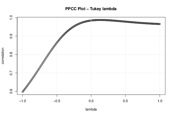
| Title produced by software | Tukey lambda PPCC Plot | ||||||||||||||||||||||||||||||||||||||||||||||||
| Date of computation | Fri, 12 Dec 2014 12:22:20 +0000 | ||||||||||||||||||||||||||||||||||||||||||||||||
| Cite this page as follows | Statistical Computations at FreeStatistics.org, Office for Research Development and Education, URL https://freestatistics.org/blog/index.php?v=date/2014/Dec/12/t1418386954yiv980wudqvcs8s.htm/, Retrieved Thu, 16 May 2024 19:58:27 +0000 | ||||||||||||||||||||||||||||||||||||||||||||||||
| Statistical Computations at FreeStatistics.org, Office for Research Development and Education, URL https://freestatistics.org/blog/index.php?pk=266594, Retrieved Thu, 16 May 2024 19:58:27 +0000 | |||||||||||||||||||||||||||||||||||||||||||||||||
| QR Codes: | |||||||||||||||||||||||||||||||||||||||||||||||||
|
| |||||||||||||||||||||||||||||||||||||||||||||||||
| Original text written by user: | |||||||||||||||||||||||||||||||||||||||||||||||||
| IsPrivate? | No (this computation is public) | ||||||||||||||||||||||||||||||||||||||||||||||||
| User-defined keywords | |||||||||||||||||||||||||||||||||||||||||||||||||
| Estimated Impact | 64 | ||||||||||||||||||||||||||||||||||||||||||||||||
Tree of Dependent Computations | |||||||||||||||||||||||||||||||||||||||||||||||||
| Family? (F = Feedback message, R = changed R code, M = changed R Module, P = changed Parameters, D = changed Data) | |||||||||||||||||||||||||||||||||||||||||||||||||
| - [Tukey lambda PPCC Plot] [Paper] [2014-12-12 12:22:20] [8c0dfc7b9b8e9dc8ad6d66876f6d8b28] [Current] | |||||||||||||||||||||||||||||||||||||||||||||||||
| Feedback Forum | |||||||||||||||||||||||||||||||||||||||||||||||||
Post a new message | |||||||||||||||||||||||||||||||||||||||||||||||||
Dataset | |||||||||||||||||||||||||||||||||||||||||||||||||
| Dataseries X: | |||||||||||||||||||||||||||||||||||||||||||||||||
-1,09842 -5,10081 0,300669 0,101669 -0,233909 2,6863 -3,86284 0,197581 -0,975839 -3,65652 -2,54314 -8,66506 -1,91624 0,339461 -1,22729 -0,610695 -4,64972 1,07758 0,220183 -1,08531 -2,77618 0,514874 -1,57337 -7,7412 -3,59165 -1,46401 -0,259212 -1,10318 -4,59588 -0,416811 0,348086 -6,44447 -4,12136 -3,77084 -4,45605 -5,4768 -6,6556 -0,589048 2,1102 -4,67029 -0,622039 -2,91384 -0,217858 -3,19751 1,88928 -4,57081 0,764804 -7,30336 -5,43595 -3,87456 -2,53739 -0,650968 0,638528 1,3834 4,61439 0,797204 2,04689 0,576657 -0,8186 -0,0331425 3,66013 3,61483 2,10601 0,980391 3,62652 2,68761 0,240096 -1,8452 2,59554 3,42243 -0,339566 5,54883 1,38969 -0,592173 -0,936289 1,73097 -1,10524 1,46812 2,92358 -1,66759 -2,59895 1,72639 -1,46938 3,74722 -1,76661 4,32574 1,40797 1,55421 2,50929 2,47847 1,22958 0,394661 1,90412 3,19377 0,959305 6,62858 5,441 0,625437 2,48092 4,01341 0,226882 1,0831 -2,6473 3,2778 3,72057 1,48615 0,451287 1,0549 1,31847 2,27233 3,16991 -0,608255 1,90658 2,72951 3,6746 1,89836 -2,60103 -0,214422 -4,58644 -0,478474 -1,00145 -1,46887 2,14995 3,50937 1,42368 1,37169 2,66742 2,58253 -0,17482 0,953009 0,151181 3,76788 3,43262 2,01818 2,3895 -2,30018 | |||||||||||||||||||||||||||||||||||||||||||||||||
Tables (Output of Computation) | |||||||||||||||||||||||||||||||||||||||||||||||||
| |||||||||||||||||||||||||||||||||||||||||||||||||
Figures (Output of Computation) | |||||||||||||||||||||||||||||||||||||||||||||||||
Input Parameters & R Code | |||||||||||||||||||||||||||||||||||||||||||||||||
| Parameters (Session): | |||||||||||||||||||||||||||||||||||||||||||||||||
| Parameters (R input): | |||||||||||||||||||||||||||||||||||||||||||||||||
| R code (references can be found in the software module): | |||||||||||||||||||||||||||||||||||||||||||||||||
gp <- function(lambda, p) | |||||||||||||||||||||||||||||||||||||||||||||||||