Repository of Reproducible Computations

Free Statistics

of Irreproducible Research!

Author's title

Author

*The author of this computation has been verified*

R Software Module

rwasp_pairs.wasp

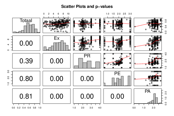
Title produced by software

Kendall tau Correlation Matrix

Date of computation

Fri, 12 Dec 2014 14:22:12 +0000

Cite this page as follows

Statistical Computations at FreeStatistics.org, Office for Research Development and Education, URL https://freestatistics.org/blog/index.php?v=date/2014/Dec/12/t1418394204dtoqfa0w3n2hzdh.htm/, Retrieved Thu, 16 May 2024 12:27:59 +0000

Statistical Computations at FreeStatistics.org, Office for Research Development and Education, URL https://freestatistics.org/blog/index.php?pk=266734, Retrieved Thu, 16 May 2024 12:27:59 +0000

QR Codes:

Paste this QR Code to cite your computation.

Original text written by user:

IsPrivate?

No (this computation is public)

User-defined keywords

Estimated Impact

Family? (F = Feedback message, R = changed R code, M = changed R Module, P = changed Parameters, D = changed Data)

-     [Multiple Regression] [] [2014-12-11 23:12:41] [02fb6cbf799bcf1e525e4e01c2f27ada]
-    D  [Multiple Regression] [] [2014-12-12 11:05:51] [02fb6cbf799bcf1e525e4e01c2f27ada]
- RMP       [Kendall tau Correlation Matrix] [] [2014-12-12 14:22:12] [ec71b09431fe59ba6fc828a3f51756a9] [Current]

Feedback Forum

Post a new message

Dataseries X:

Download CSV

Histogram

Boxplots

0.56 7.5 1.8 2.1 1.5
0.79 2.5 1.6 1.5 1.8
0.68 6.0 2.1 2.0 2.1
0.66 6.5 2.2 2.0 2.1
0.37 1.0 2.3 2.1 1.9
0.71 1.0 2.1 2.0 1.6
0.35 5.5 2.7 2.3 2.1
0.55 8.5 2.1 2.1 2.1
0.76 6.5 2.4 2.1 2.2
0.49 4.5 2.9 2.2 1.5
0.56 2.0 2.2 2.1 1.9
0.60 5.0 2.1 2.1 2.2
0.44 0.5 2.2 2.1 1.6
0.55 5.0 2.2 2.0 1.5
0.58 5.0 2.7 2.3 1.9
0.40 2.5 1.9 1.8 0.1
0.42 5.0 2.0 2.0 2.2
0.58 5.5 2.5 2.2 1.8
0.64 3.5 2.2 2.0 1.6
0.58 3.0 2.3 2.1 2.2
0.44 4.0 1.9 2.0 2.1
0.46 0.5 2.1 1.8 1.9
0.64 6.5 3.5 2.2 1.6
0.59 4.5 2.1 2.2 1.9
0.54 7.5 2.3 1.7 2.2
0.71 5.5 2.3 2.1 1.8
0.20 4.0 2.2 2.3 2.4
0.89 7.5 3.5 2.7 2.4
0.55 7.0 1.9 1.9 2.5
0.71 4.0 1.9 2.0 1.9
0.48 5.5 1.9 2.0 2.1
0.49 2.5 1.9 1.9 1.9
0.58 5.5 2.1 2.0 2.1
0.78 0.5 1.6 2.0 1.9
0.71 3.5 2.0 2.0 1.5
0.51 2.5 3.2 2.1 1.9
0.65 4.5 2.3 2.0 2.1
0.68 4.5 2.5 1.8 1.5
0.24 4.5 1.8 2.0 2.1
0.36 6.0 2.4 2.2 2.1
0.65 2.5 2.8 2.2 1.8
0.79 5.0 2.3 2.1 2.4
0.67 0.0 2.0 1.8 2.1
0.74 5.0 2.5 1.9 1.9
0.72 6.5 2.3 2.1 2.1
0.73 5.0 1.8 2.0 1.9
0.58 6.0 1.9 1.9 2.4
0.67 4.5 2.6 2.2 2.1
0.43 5.5 2.0 2.0 2.2
0.59 1.0 2.6 2.0 2.2
0.43 7.5 1.6 1.7 1.8
0.80 6.0 2.2 2.0 2.1
0.74 5.0 2.1 2.2 2.4
0.43 1.0 1.8 1.7 2.2
0.72 5.0 1.8 2.0 2.1
0.50 6.5 1.9 2.2 1.5
0.45 7.0 2.4 2.0 1.9
0.88 4.5 1.9 1.9 1.8
0.67 0.0 2.0 2.0 1.8
0.32 8.5 2.1 2.0 1.6
0.20 3.5 1.7 1.6 1.2
0.84 7.5 1.9 2.1 1.8
0.83 3.5 2.1 2.1 1.5
0.65 6.0 2.4 2.0 2.1
0.74 1.5 1.8 1.9 2.4
0.53 9.0 2.3 2.2 2.4
0.58 3.5 2.1 2.1 1.5
0.65 3.5 2.0 1.8 1.8
0.64 4.0 2.8 2.3 2.1
0.60 6.5 2.0 2.3 2.2
0.52 7.5 2.7 2.2 2.1
0.53 6.0 2.1 2.1 1.9
0.73 5.0 2.9 2.2 2.1
0.52 5.5 2.0 1.9 1.9
0.61 3.5 1.8 1.8 1.6
0.73 7.5 2.6 2.1 2.4
0.79 1.0 2.5 1.8 1.9
0.29 6.5 2.1 2.0 1.9
0.86 NA 2.3 1.7 1.9
0.37 6.5 2.3 2.1 2.1
0.68 6.5 2.2 2.1 1.8
0.52 7.0 2.0 2.1 2.1
0.26 3.5 2.2 1.8 2.4
0.74 1.5 2.1 2.0 2.1
0.72 4.0 2.1 2.1 2.2
0.24 7.5 1.9 1.9 2.1
0.71 4.5 2.0 2.1 2.2
0.59 0.0 1.7 1.0 1.6
0.27 3.5 2.2 2.2 2.4
0.57 5.5 2.2 2.1 2.1
0.51 5.0 2.3 1.9 1.9
0.69 4.5 2.4 2.0 2.4
0.69 2.5 2.1 1.9 2.1
0.50 7.5 1.9 2.0 1.8
0.63 7.0 1.7 1.8 2.1
0.65 0.0 1.8 2.0 1.8
0.54 4.5 1.5 2.0 1.9
0.69 3.0 1.9 2.0 1.9
0.52 1.5 1.9 1.8 2.4
0.53 3.5 1.7 2.0 1.8
0.74 2.5 1.9 1.1 1.8
0.73 5.5 1.9 1.8 2.1
0.75 8.0 1.8 1.8 2.1
0.70 1.0 2.4 2.0 2.4
0.69 5.0 1.8 1.9 1.9
0.57 4.5 1.9 2.1 1.8
0.14 3.0 1.8 1.6 1.8
0.42 3.0 2.1 2.2 2.2
0.48 8.0 1.9 1.9 2.4
0.27 2.5 2.2 2.0 1.8
0.21 7.0 2.0 2.1 2.4
0.41 0.0 1.7 1.3 1.8
0.56 1.0 1.7 1.8 1.9
0.44 3.5 1.8 1.9 2.4
0.52 5.5 1.9 2.1 2.1
0.59 5.5 1.8 1.8 1.9
0.73 0.5 1 0.75 2.1
0.79 7.5 1 1.5 2.7
0.67 9 4 3 2.1
0.88 9.5 4 2.25 2.1
0.96 8.5 3 3 2.1
0.43 7 2 1.5 2.1
0.84 8 4 3 2.1
0.81 10 4 3 2.1
0.67 7 4 3 2.1
0.45 8.5 2 0.75 2.1
0.58 9 4 3 2.4
0.70 9.5 1 2.25 1.95
0.61 4 3 1.5 2.1
0.44 6 3 1.5 2.1
0.54 8 4 2.25 1.95
0.41 5.5 3 3 2.1
0.66 9.5 4 3 2.4
0.83 7.5 3 1.5 2.1
0.88 7 3 2.25 2.25
0.40 7.5 4 2.25 2.4
0.54 8 3 1.5 2.25
0.60 7 3 2.25 2.55
0.57 7 2 1.5 1.95
0.59 6 2 2.25 2.4
0.81 10 3 2.25 2.1
0.51 2.5 1 3 2.1
0.65 9 4 3 2.4
0.59 8 3 3 2.1
0.68 6 2 1.5 2.1
0.65 8.5 4 3 2.25
0.06 6 4 3 2.25
0.74 9 4 2.25 2.4
0.29 8 4 1.5 2.1
0.73 8 4 2.25 2.1
0.54 9 4 2.25 2.4
0.39 5.5 3 3 2.1
0.27 5 4 0.75 1.95
0.40 7 3 2.25 2.1
0.20 5.5 4 3 2.25
0.85 9 4 3 2.25
0.42 2 4 1.5 2.4
0.68 8.5 3 2.25 2.25
0.72 9 4 3 2.25
0.52 8.5 4 2.25 2.1
0.78 9 2 1.5 2.1
0.60 7.5 2 2.25 2.1
0.93 10 4 2.25 2.7
0.73 9 3 1.5 2.1
0.81 7.5 3 2.25 2.1
0.51 6 2 1.5 2.25
0.86 10.5 3 2.25 2.7
0.67 8.5 2 3 2.4
0.50 8 4 3 2.1
0.74 10 1 3 2.1
0.85 10.5 4 3 2.4
0.75 6.5 1 1.5 1.95
0.83 9.5 4 2.25 2.7
0.82 8.5 3 1.5 2.1
0.58 7.5 3 2.25 2.25
0.72 5 2 2.25 2.1
0.89 8 3 2.25 2.7
0.51 10 3 3 2.1
0.75 7 4 1.5 2.1
0.84 7.5 4 2.25 1.65
0.84 7.5 4 2.25 1.65
0.59 9.5 3 3 2.1
0.64 6 3 2.25 2.1
0.45 10 4 3 2.1
0.57 7 4 2.25 2.1
0.58 3 1 1.5 2.1
0.72 6 2 3 2.4
0.38 7 3 1.5 2.4
0.68 10 4 3 2.1
0.45 7 3 3 2.25
0.55 3.5 4 3 2.4
0.73 8 3 3 2.1
0.73 10 3 2.25 2.1
0.73 5.5 3 2.25 2.4
0.71 6 3 0.75 2.4
0.38 6.5 1 3 2.1
0.79 6.5 1 0.75 2.1
0.32 8.5 3 1.5 2.4
0.62 4 2 1.5 2.1
0.42 9.5 3 3 2.7
0.45 8 2 1.5 2.1
0.97 8.5 2 2.25 2.1
0.67 5.5 4 3 2.25
0.08 7 2 3 2.1
0.49 9 2 1.5 2.4
0.66 8 3 3 2.25
0.67 10 4 3 2.25
0.55 8 2 1.5 2.1
0.55 6 4 1.5 2.1
0.49 8 3 2.25 2.4
0.56 5 4 1.5 2.25
0.69 9 2 1.5 2.1
0.47 4.5 1 2.25 2.1
0.68 8.5 1 1.5 1.65
0.43 7 1 2.25 1.65
0.00 9.5 4 3 2.7
0.48 8.5 3 3 2.1
0.77 7.5 1 0.75 1.95
0.71 7.5 4 1.5 2.25
0.43 5 3 1.5 2.4
0.50 7 2 2.25 1.95
0.68 8 4 2.25 2.1
0.34 5.5 3 1.5 2.4
0.47 8.5 3 2.25 2.1
0.33 7.5 4 0.75 2.1
0.80 9.5 4 2.25 2.4
0.74 7 1 0.75 2.4
0.82 8 3 2.25 2.4
0.57 8.5 4 3 2.25
0.46 3.5 1 0.75 2.4
0.91 6.5 3 0.75 2.1
0.41 6.5 4 3 2.1
0.64 10.5 4 3 1.8
0.58 8.5 1 3 2.7
0.45 8 4 3 2.1
0.77 10 2 1.5 2.1
0.67 10 3 3 2.4
0.53 9.5 4 3 2.55
0.07 9 4 3 2.55
0.65 10 4 3 2.1
0.76 7.5 2 1.5 2.1
0.56 4.5 4 2.25 2.1
0.07 4.5 2 0.75 2.25
0.72 0.5 1 0.75 2.25
0.61 6.5 1 2.25 2.1
0.47 4.5 4 3 2.1
0.06 5.5 2 2.25 1.95
0.37 5 2 3 2.4
0.76 6 3 2.25 2.1
0.47 4 2 3 2.4
0.55 8 3 1.5 2.4
0.85 10.5 4 3 2.4
0.77 8.5 4 3 2.25
0.79 6.5 2 0.75 1.95
0.70 8 3 1.5 2.1
0.46 8.5 4 3 2.1
0.51 5.5 3 3 2.55
0.65 7 4 3 2.1
0.57 5 4 2.25 2.1
0.68 3.5 4 2.25 2.1
0.52 5 2 3 1.95
0.70 9 2 1.5 2.25
0.46 8.5 2 2.25 2.4
0.88 5 4 2.25 1.95
0.76 9.5 3 2.25 2.1
0.74 3 2 0.75 2.1
0.56 1.5 2 2.25 1.95
0.47 6 3 1.5 2.1
0.44 0.5 3 2.25 2.1
0.75 6.5 1 1.5 1.95
0.78 7.5 2 0.75 2.1
0.26 4.5 2 1.5 1.95
0.55 8 3 1.5 2.4
0.49 9 3 2.25 2.4
0.81 7.5 2 1.5 2.4
0.45 8.5 2 1.5 1.95
0.39 7 3 3 2.7
0.89 9.5 3 2.25 2.1
0.66 6.5 1 1.5 1.95
0.34 9.5 3 0.75 2.1
0.84 6 2 2.25 1.95
0.05 8 2 3 2.1
0.79 9.5 3 3 2.25
0.60 8 3 1.5 2.7
0.69 8 3 1.5 2.1
0.58 9 3 2.25 2.4
0.66 5 1 0.75 1.35

Summary of computational transaction
Raw Input	view raw input (R code)
Raw Output	view raw output of R engine
Computing time	2 seconds
R Server	'Gwilym Jenkins' @ jenkins.wessa.net

\begin{tabular}{lllllllll}
\hline
Summary of computational transaction \tabularnewline
Raw Input & view raw input (R code)  \tabularnewline
Raw Output & view raw output of R engine  \tabularnewline
Computing time & 2 seconds \tabularnewline
R Server & 'Gwilym Jenkins' @ jenkins.wessa.net \tabularnewline
\hline
\end{tabular}
%Source: https://freestatistics.org/blog/index.php?pk=266734&T=0

[TABLE]
[ROW][C]Summary of computational transaction[/C][/ROW]
[ROW][C]Raw Input[/C][C]view raw input (R code) [/C][/ROW]
[ROW][C]Raw Output[/C][C]view raw output of R engine [/C][/ROW]
[ROW][C]Computing time[/C][C]2 seconds[/C][/ROW]
[ROW][C]R Server[/C][C]'Gwilym Jenkins' @ jenkins.wessa.net[/C][/ROW]
[/TABLE]
Source: https://freestatistics.org/blog/index.php?pk=266734&T=0

Globally Unique Identifier (entire table): ba.freestatistics.org/blog/index.php?pk=266734&T=0

As an alternative you can also use a QR Code:

The GUIDs for individual cells are displayed in the table below:

Summary of computational transaction
Raw Input	view raw input (R code)
Raw Output	view raw output of R engine
Computing time	2 seconds
R Server	'Gwilym Jenkins' @ jenkins.wessa.net

Correlations for all pairs of data series (method=kendall)
	Totaal	Ex	PR	PE	PA
Totaal	1	0.123	0.036	-0.011	-0.011
Ex	0.123	1	0.311	0.247	0.265
PR	0.036	0.311	1	0.383	0.245
PE	-0.011	0.247	0.383	1	0.171
PA	-0.011	0.265	0.245	0.171	1

\begin{tabular}{lllllllll}
\hline
Correlations for all pairs of data series (method=kendall) \tabularnewline
  & Totaal & Ex & PR & PE & PA \tabularnewline
Totaal & 1 & 0.123 & 0.036 & -0.011 & -0.011 \tabularnewline
Ex & 0.123 & 1 & 0.311 & 0.247 & 0.265 \tabularnewline
PR & 0.036 & 0.311 & 1 & 0.383 & 0.245 \tabularnewline
PE & -0.011 & 0.247 & 0.383 & 1 & 0.171 \tabularnewline
PA & -0.011 & 0.265 & 0.245 & 0.171 & 1 \tabularnewline
\hline
\end{tabular}
%Source: https://freestatistics.org/blog/index.php?pk=266734&T=1

[TABLE]
[ROW][C]Correlations for all pairs of data series (method=kendall)[/C][/ROW]
[ROW][C] [/C][C]Totaal[/C][C]Ex[/C][C]PR[/C][C]PE[/C][C]PA[/C][/ROW]
[ROW][C]Totaal[/C][C]1[/C][C]0.123[/C][C]0.036[/C][C]-0.011[/C][C]-0.011[/C][/ROW]
[ROW][C]Ex[/C][C]0.123[/C][C]1[/C][C]0.311[/C][C]0.247[/C][C]0.265[/C][/ROW]
[ROW][C]PR[/C][C]0.036[/C][C]0.311[/C][C]1[/C][C]0.383[/C][C]0.245[/C][/ROW]
[ROW][C]PE[/C][C]-0.011[/C][C]0.247[/C][C]0.383[/C][C]1[/C][C]0.171[/C][/ROW]
[ROW][C]PA[/C][C]-0.011[/C][C]0.265[/C][C]0.245[/C][C]0.171[/C][C]1[/C][/ROW]
[/TABLE]
Source: https://freestatistics.org/blog/index.php?pk=266734&T=1

Globally Unique Identifier (entire table): ba.freestatistics.org/blog/index.php?pk=266734&T=1

As an alternative you can also use a QR Code:

The GUIDs for individual cells are displayed in the table below:

Correlations for all pairs of data series (method=kendall)
	Totaal	Ex	PR	PE	PA
Totaal	1	0.123	0.036	-0.011	-0.011
Ex	0.123	1	0.311	0.247	0.265
PR	0.036	0.311	1	0.383	0.245
PE	-0.011	0.247	0.383	1	0.171
PA	-0.011	0.265	0.245	0.171	1

Correlations for all pairs of data series with p-values
pair	Pearson r	Spearman rho	Kendall tau
Totaal;Ex	0.1451	0.1793	0.1232
p-value	(0.0141)	(0.0023)	(0.0027)
Totaal;PR	0.0419	0.0514	0.036
p-value	(0.4795)	(0.3852)	(0.3928)
Totaal;PE	-0.0483	-0.0167	-0.0107
p-value	(0.4155)	(0.7785)	(0.8001)
Totaal;PA	0.0072	-0.014	-0.0105
p-value	(0.9029)	(0.8137)	(0.8065)
Ex;PR	0.4059	0.4182	0.3112
p-value	(0)	(0)	(0)
Ex;PE	0.3029	0.3338	0.2468
p-value	(0)	(0)	(0)
Ex;PA	0.3477	0.3483	0.2648
p-value	(0)	(0)	(0)
PR;PE	0.4369	0.4655	0.383
p-value	(0)	(0)	(0)
PR;PA	0.2744	0.322	0.2453
p-value	(0)	(0)	(0)
PE;PA	0.1994	0.2288	0.171
p-value	(7e-04)	(1e-04)	(2e-04)

\begin{tabular}{lllllllll}
\hline
Correlations for all pairs of data series with p-values \tabularnewline
pair & Pearson r & Spearman rho & Kendall tau \tabularnewline
Totaal;Ex & 0.1451 & 0.1793 & 0.1232 \tabularnewline
p-value & (0.0141) & (0.0023) & (0.0027) \tabularnewline
Totaal;PR & 0.0419 & 0.0514 & 0.036 \tabularnewline
p-value & (0.4795) & (0.3852) & (0.3928) \tabularnewline
Totaal;PE & -0.0483 & -0.0167 & -0.0107 \tabularnewline
p-value & (0.4155) & (0.7785) & (0.8001) \tabularnewline
Totaal;PA & 0.0072 & -0.014 & -0.0105 \tabularnewline
p-value & (0.9029) & (0.8137) & (0.8065) \tabularnewline
Ex;PR & 0.4059 & 0.4182 & 0.3112 \tabularnewline
p-value & (0) & (0) & (0) \tabularnewline
Ex;PE & 0.3029 & 0.3338 & 0.2468 \tabularnewline
p-value & (0) & (0) & (0) \tabularnewline
Ex;PA & 0.3477 & 0.3483 & 0.2648 \tabularnewline
p-value & (0) & (0) & (0) \tabularnewline
PR;PE & 0.4369 & 0.4655 & 0.383 \tabularnewline
p-value & (0) & (0) & (0) \tabularnewline
PR;PA & 0.2744 & 0.322 & 0.2453 \tabularnewline
p-value & (0) & (0) & (0) \tabularnewline
PE;PA & 0.1994 & 0.2288 & 0.171 \tabularnewline
p-value & (7e-04) & (1e-04) & (2e-04) \tabularnewline
\hline
\end{tabular}
%Source: https://freestatistics.org/blog/index.php?pk=266734&T=2

[TABLE]
[ROW][C]Correlations for all pairs of data series with p-values[/C][/ROW]
[ROW][C]pair[/C][C]Pearson r[/C][C]Spearman rho[/C][C]Kendall tau[/C][/ROW]
[ROW][C]Totaal;Ex[/C][C]0.1451[/C][C]0.1793[/C][C]0.1232[/C][/ROW]
[ROW][C]p-value[/C][C](0.0141)[/C][C](0.0023)[/C][C](0.0027)[/C][/ROW]
[ROW][C]Totaal;PR[/C][C]0.0419[/C][C]0.0514[/C][C]0.036[/C][/ROW]
[ROW][C]p-value[/C][C](0.4795)[/C][C](0.3852)[/C][C](0.3928)[/C][/ROW]
[ROW][C]Totaal;PE[/C][C]-0.0483[/C][C]-0.0167[/C][C]-0.0107[/C][/ROW]
[ROW][C]p-value[/C][C](0.4155)[/C][C](0.7785)[/C][C](0.8001)[/C][/ROW]
[ROW][C]Totaal;PA[/C][C]0.0072[/C][C]-0.014[/C][C]-0.0105[/C][/ROW]
[ROW][C]p-value[/C][C](0.9029)[/C][C](0.8137)[/C][C](0.8065)[/C][/ROW]
[ROW][C]Ex;PR[/C][C]0.4059[/C][C]0.4182[/C][C]0.3112[/C][/ROW]
[ROW][C]p-value[/C][C](0)[/C][C](0)[/C][C](0)[/C][/ROW]
[ROW][C]Ex;PE[/C][C]0.3029[/C][C]0.3338[/C][C]0.2468[/C][/ROW]
[ROW][C]p-value[/C][C](0)[/C][C](0)[/C][C](0)[/C][/ROW]
[ROW][C]Ex;PA[/C][C]0.3477[/C][C]0.3483[/C][C]0.2648[/C][/ROW]
[ROW][C]p-value[/C][C](0)[/C][C](0)[/C][C](0)[/C][/ROW]
[ROW][C]PR;PE[/C][C]0.4369[/C][C]0.4655[/C][C]0.383[/C][/ROW]
[ROW][C]p-value[/C][C](0)[/C][C](0)[/C][C](0)[/C][/ROW]
[ROW][C]PR;PA[/C][C]0.2744[/C][C]0.322[/C][C]0.2453[/C][/ROW]
[ROW][C]p-value[/C][C](0)[/C][C](0)[/C][C](0)[/C][/ROW]
[ROW][C]PE;PA[/C][C]0.1994[/C][C]0.2288[/C][C]0.171[/C][/ROW]
[ROW][C]p-value[/C][C](7e-04)[/C][C](1e-04)[/C][C](2e-04)[/C][/ROW]
[/TABLE]
Source: https://freestatistics.org/blog/index.php?pk=266734&T=2

Globally Unique Identifier (entire table): ba.freestatistics.org/blog/index.php?pk=266734&T=2

As an alternative you can also use a QR Code:

The GUIDs for individual cells are displayed in the table below:

Correlations for all pairs of data series with p-values
pair	Pearson r	Spearman rho	Kendall tau
Totaal;Ex	0.1451	0.1793	0.1232
p-value	(0.0141)	(0.0023)	(0.0027)
Totaal;PR	0.0419	0.0514	0.036
p-value	(0.4795)	(0.3852)	(0.3928)
Totaal;PE	-0.0483	-0.0167	-0.0107
p-value	(0.4155)	(0.7785)	(0.8001)
Totaal;PA	0.0072	-0.014	-0.0105
p-value	(0.9029)	(0.8137)	(0.8065)
Ex;PR	0.4059	0.4182	0.3112
p-value	(0)	(0)	(0)
Ex;PE	0.3029	0.3338	0.2468
p-value	(0)	(0)	(0)
Ex;PA	0.3477	0.3483	0.2648
p-value	(0)	(0)	(0)
PR;PE	0.4369	0.4655	0.383
p-value	(0)	(0)	(0)
PR;PA	0.2744	0.322	0.2453
p-value	(0)	(0)	(0)
PE;PA	0.1994	0.2288	0.171
p-value	(7e-04)	(1e-04)	(2e-04)

Meta Analysis of Correlation Tests
Number of significant by total number of Correlations
Type I error	Pearson r	Spearman rho	Kendall tau
0.01	0.6	0.7	0.7
0.02	0.7	0.7	0.7
0.03	0.7	0.7	0.7
0.04	0.7	0.7	0.7
0.05	0.7	0.7	0.7
0.06	0.7	0.7	0.7
0.07	0.7	0.7	0.7
0.08	0.7	0.7	0.7
0.09	0.7	0.7	0.7
0.1	0.7	0.7	0.7

\begin{tabular}{lllllllll}
\hline
Meta Analysis of Correlation Tests \tabularnewline
Number of significant by total number of Correlations \tabularnewline
Type I error & Pearson r & Spearman rho & Kendall tau \tabularnewline
0.01 & 0.6 & 0.7 & 0.7 \tabularnewline
0.02 & 0.7 & 0.7 & 0.7 \tabularnewline
0.03 & 0.7 & 0.7 & 0.7 \tabularnewline
0.04 & 0.7 & 0.7 & 0.7 \tabularnewline
0.05 & 0.7 & 0.7 & 0.7 \tabularnewline
0.06 & 0.7 & 0.7 & 0.7 \tabularnewline
0.07 & 0.7 & 0.7 & 0.7 \tabularnewline
0.08 & 0.7 & 0.7 & 0.7 \tabularnewline
0.09 & 0.7 & 0.7 & 0.7 \tabularnewline
0.1 & 0.7 & 0.7 & 0.7 \tabularnewline
\hline
\end{tabular}
%Source: https://freestatistics.org/blog/index.php?pk=266734&T=3

[TABLE]
[ROW][C]Meta Analysis of Correlation Tests[/C][/ROW]
[ROW][C]Number of significant by total number of Correlations[/C][/ROW]
[ROW][C]Type I error[/C][C]Pearson r[/C][C]Spearman rho[/C][C]Kendall tau[/C][/ROW]
[ROW][C]0.01[/C][C]0.6[/C][C]0.7[/C][C]0.7[/C][/ROW]
[ROW][C]0.02[/C][C]0.7[/C][C]0.7[/C][C]0.7[/C][/ROW]
[ROW][C]0.03[/C][C]0.7[/C][C]0.7[/C][C]0.7[/C][/ROW]
[ROW][C]0.04[/C][C]0.7[/C][C]0.7[/C][C]0.7[/C][/ROW]
[ROW][C]0.05[/C][C]0.7[/C][C]0.7[/C][C]0.7[/C][/ROW]
[ROW][C]0.06[/C][C]0.7[/C][C]0.7[/C][C]0.7[/C][/ROW]
[ROW][C]0.07[/C][C]0.7[/C][C]0.7[/C][C]0.7[/C][/ROW]
[ROW][C]0.08[/C][C]0.7[/C][C]0.7[/C][C]0.7[/C][/ROW]
[ROW][C]0.09[/C][C]0.7[/C][C]0.7[/C][C]0.7[/C][/ROW]
[ROW][C]0.1[/C][C]0.7[/C][C]0.7[/C][C]0.7[/C][/ROW]
[/TABLE]
Source: https://freestatistics.org/blog/index.php?pk=266734&T=3

Globally Unique Identifier (entire table): ba.freestatistics.org/blog/index.php?pk=266734&T=3

As an alternative you can also use a QR Code:

The GUIDs for individual cells are displayed in the table below:

Meta Analysis of Correlation Tests
Number of significant by total number of Correlations
Type I error	Pearson r	Spearman rho	Kendall tau
0.01	0.6	0.7	0.7
0.02	0.7	0.7	0.7
0.03	0.7	0.7	0.7
0.04	0.7	0.7	0.7
0.05	0.7	0.7	0.7
0.06	0.7	0.7	0.7
0.07	0.7	0.7	0.7
0.08	0.7	0.7	0.7
0.09	0.7	0.7	0.7
0.1	0.7	0.7	0.7

Figure 1

PNG link

Postscript link

PDF link

Parameters (Session):

Parameters (R input):

par1 = kendall ;

R code (references can be found in the software module):

panel.tau <- function(x, y, digits=2, prefix='', cex.cor)
{
usr <- par('usr'); on.exit(par(usr))
par(usr = c(0, 1, 0, 1))
rr <- cor.test(x, y, method=par1)
r <- round(rr$p.value,2)
txt <- format(c(r, 0.123456789), digits=digits)[1]
txt <- paste(prefix, txt, sep='')
if(missing(cex.cor)) cex <- 0.5/strwidth(txt)
text(0.5, 0.5, txt, cex = cex)
}
panel.hist <- function(x, ...)
{
usr <- par('usr'); on.exit(par(usr))
par(usr = c(usr[1:2], 0, 1.5) )
h <- hist(x, plot = FALSE)
breaks <- h$breaks; nB <- length(breaks)
y <- h$counts; y <- y/max(y)
rect(breaks[-nB], 0, breaks[-1], y, col='grey', ...)
}
bitmap(file='test1.png')
pairs(t(y),diag.panel=panel.hist, upper.panel=panel.smooth, lower.panel=panel.tau, main=main)
dev.off()
load(file='createtable')
n <- length(y[,1])
n
a<-table.start()
a<-table.row.start(a)
a<-table.element(a,paste('Correlations for all pairs of data series (method=',par1,')',sep=''),n+1,TRUE)
a<-table.row.end(a)
a<-table.row.start(a)
a<-table.element(a,' ',header=TRUE)
for (i in 1:n) {
a<-table.element(a,dimnames(t(x))[[2]][i],header=TRUE)
}
a<-table.row.end(a)
for (i in 1:n) {
a<-table.row.start(a)
a<-table.element(a,dimnames(t(x))[[2]][i],header=TRUE)
for (j in 1:n) {
r <- cor.test(y[i,],y[j,],method=par1)
a<-table.element(a,round(r$estimate,3))
}
a<-table.row.end(a)
}
a<-table.end(a)
table.save(a,file='mytable.tab')
ncorrs <- (n*n -n)/2
mycorrs <- array(0, dim=c(10,3))
a<-table.start()
a<-table.row.start(a)
a<-table.element(a,'Correlations for all pairs of data series with p-values',4,TRUE)
a<-table.row.end(a)
a<-table.row.start(a)
a<-table.element(a,'pair',1,TRUE)
a<-table.element(a,'Pearson r',1,TRUE)
a<-table.element(a,'Spearman rho',1,TRUE)
a<-table.element(a,'Kendall tau',1,TRUE)
a<-table.row.end(a)
cor.test(y[1,],y[2,],method=par1)
for (i in 1:(n-1))
{
for (j in (i+1):n)
{
a<-table.row.start(a)
dum <- paste(dimnames(t(x))[[2]][i],';',dimnames(t(x))[[2]][j],sep='')
a<-table.element(a,dum,header=TRUE)
rp <- cor.test(y[i,],y[j,],method='pearson')
a<-table.element(a,round(rp$estimate,4))
rs <- cor.test(y[i,],y[j,],method='spearman')
a<-table.element(a,round(rs$estimate,4))
rk <- cor.test(y[i,],y[j,],method='kendall')
a<-table.element(a,round(rk$estimate,4))
a<-table.row.end(a)
a<-table.row.start(a)
a<-table.element(a,'p-value',header=T)
a<-table.element(a,paste('(',round(rp$p.value,4),')',sep=''))
a<-table.element(a,paste('(',round(rs$p.value,4),')',sep=''))
a<-table.element(a,paste('(',round(rk$p.value,4),')',sep=''))
a<-table.row.end(a)
for (iii in 1:10) {
iiid100 <- iii / 100
if (rp$p.value < iiid100) mycorrs[iii, 1] = mycorrs[iii, 1] + 1
if (rs$p.value < iiid100) mycorrs[iii, 2] = mycorrs[iii, 2] + 1
if (rk$p.value < iiid100) mycorrs[iii, 3] = mycorrs[iii, 3] + 1
}
}
}
a<-table.end(a)
table.save(a,file='mytable1.tab')
a<-table.start()
a<-table.row.start(a)
a<-table.element(a,'Meta Analysis of Correlation Tests',4,TRUE)
a<-table.row.end(a)
a<-table.row.start(a)
a<-table.element(a,'Number of significant by total number of Correlations',4,TRUE)
a<-table.row.end(a)
a<-table.row.start(a)
a<-table.element(a,'Type I error',1,TRUE)
a<-table.element(a,'Pearson r',1,TRUE)
a<-table.element(a,'Spearman rho',1,TRUE)
a<-table.element(a,'Kendall tau',1,TRUE)
a<-table.row.end(a)
for (iii in 1:10) {
iiid100 <- iii / 100
a<-table.row.start(a)
a<-table.element(a,round(iiid100,2),header=T)
a<-table.element(a,round(mycorrs[iii,1]/ncorrs,2))
a<-table.element(a,round(mycorrs[iii,2]/ncorrs,2))
a<-table.element(a,round(mycorrs[iii,3]/ncorrs,2))
a<-table.row.end(a)
}
a<-table.end(a)
table.save(a,file='mytable2.tab')

Free Statistics

Description of Statistical Computation

Tree of Dependent Computations

Dataset

Tables (Output of Computation)

Figures (Output of Computation)

Input Parameters & R Code