Free Statistics
of Irreproducible Research!
Description of Statistical Computation | |||||||||||||||||||||||||||||||||||||||||||||||||||||||||||||||||||||||||||||||||
|---|---|---|---|---|---|---|---|---|---|---|---|---|---|---|---|---|---|---|---|---|---|---|---|---|---|---|---|---|---|---|---|---|---|---|---|---|---|---|---|---|---|---|---|---|---|---|---|---|---|---|---|---|---|---|---|---|---|---|---|---|---|---|---|---|---|---|---|---|---|---|---|---|---|---|---|---|---|---|---|---|---|
| Author's title | |||||||||||||||||||||||||||||||||||||||||||||||||||||||||||||||||||||||||||||||||
| Author | *The author of this computation has been verified* | ||||||||||||||||||||||||||||||||||||||||||||||||||||||||||||||||||||||||||||||||
| R Software Module | rwasp_notchedbox1.wasp | ||||||||||||||||||||||||||||||||||||||||||||||||||||||||||||||||||||||||||||||||
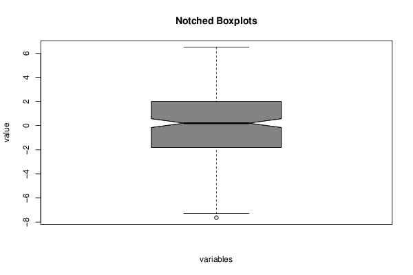
| Title produced by software | Notched Boxplots | ||||||||||||||||||||||||||||||||||||||||||||||||||||||||||||||||||||||||||||||||
| Date of computation | Sat, 13 Dec 2014 10:20:12 +0000 | ||||||||||||||||||||||||||||||||||||||||||||||||||||||||||||||||||||||||||||||||
| Cite this page as follows | Statistical Computations at FreeStatistics.org, Office for Research Development and Education, URL https://freestatistics.org/blog/index.php?v=date/2014/Dec/13/t141846637654dyg8oxxbcjd2c.htm/, Retrieved Thu, 16 May 2024 23:51:01 +0000 | ||||||||||||||||||||||||||||||||||||||||||||||||||||||||||||||||||||||||||||||||
| Statistical Computations at FreeStatistics.org, Office for Research Development and Education, URL https://freestatistics.org/blog/index.php?pk=266944, Retrieved Thu, 16 May 2024 23:51:01 +0000 | |||||||||||||||||||||||||||||||||||||||||||||||||||||||||||||||||||||||||||||||||
| QR Codes: | |||||||||||||||||||||||||||||||||||||||||||||||||||||||||||||||||||||||||||||||||
|
| |||||||||||||||||||||||||||||||||||||||||||||||||||||||||||||||||||||||||||||||||
| Original text written by user: | |||||||||||||||||||||||||||||||||||||||||||||||||||||||||||||||||||||||||||||||||
| IsPrivate? | No (this computation is public) | ||||||||||||||||||||||||||||||||||||||||||||||||||||||||||||||||||||||||||||||||
| User-defined keywords | |||||||||||||||||||||||||||||||||||||||||||||||||||||||||||||||||||||||||||||||||
| Estimated Impact | 106 | ||||||||||||||||||||||||||||||||||||||||||||||||||||||||||||||||||||||||||||||||
Tree of Dependent Computations | |||||||||||||||||||||||||||||||||||||||||||||||||||||||||||||||||||||||||||||||||
| Family? (F = Feedback message, R = changed R code, M = changed R Module, P = changed Parameters, D = changed Data) | |||||||||||||||||||||||||||||||||||||||||||||||||||||||||||||||||||||||||||||||||
| - [Notched Boxplots] [boxplot] [2014-12-13 10:20:12] [0e510e249d31411b3faa1a25774a526d] [Current] | |||||||||||||||||||||||||||||||||||||||||||||||||||||||||||||||||||||||||||||||||
| Feedback Forum | |||||||||||||||||||||||||||||||||||||||||||||||||||||||||||||||||||||||||||||||||
Post a new message | |||||||||||||||||||||||||||||||||||||||||||||||||||||||||||||||||||||||||||||||||
Dataset | |||||||||||||||||||||||||||||||||||||||||||||||||||||||||||||||||||||||||||||||||
| Dataseries X: | |||||||||||||||||||||||||||||||||||||||||||||||||||||||||||||||||||||||||||||||||
0.238497 0.677948 -0.0734505 -4.84141 -4.86438 -2.11042 1.85739 0.811498 -0.863432 -6.35877 -1.40974 -7.63684 -0.466661 -1.61276 -3.53005 -0.0635677 -1.5002 -3.08476 -2.65208 -1.39036 -4.77135 1.09576 -2.90497 2.01284 -1.0898 -3.1862 2.56872 1.7199 -1.30814 -0.537623 -3.44826 -2.27305 -3.27134 -3.9693 -1.4717 -2.32228 -1.10164 0.502923 -3.0886 -2.84213 -4.94242 -2.49517 1.32205 -1.40908 2.36735 -2.74775 -0.291801 -2.72799 2.60663 1.44313 -0.0444277 -3.98173 -2.01987 -0.223526 0.201302 -3.23044 -6.19629 2.57902 -1.20028 1.32292 -3.73772 0.337026 -3.60925 2.27981 -2.96027 -1.3184 -3.1453 -0.537491 2.05375 0.959101 -2.01619 -0.267122 -3.23586 3.29307 0.0274524 -0.713411 1.27009 -1.82426 -0.945416 -3.54579 -0.530508 3.04491 -1.09802 -5.52218 -0.761055 0.205994 1.07081 0.432805 -2.14822 2.08272 2.23458 -5.37548 -1.28443 -3.67677 -3.79013 -1.743 -5.17052 0.406295 2.21755 -2.42132 0.052157 -1.40026 -0.849827 -0.773986 2.82165 -1.83632 2.8179 -5.66283 -4.06326 -1.19071 0.516917 0.981162 -5.52594 0.4299 3.64473 2.92095 -0.231366 2.83157 -5.10806 3.13865 -1.97164 2.53744 0.233905 4.12487 -3.67276 -0.394087 1.49508 -2.63859 3.13736 1.70794 2.37283 -1.93119 2.25982 1.35725 0.624398 -1.6862 3.73113 -2.86881 0.61557 -1.82686 0.470194 6.48779 2.96647 1.986 1.38565 2.09278 0.833716 0.794506 -2.79697 1.71911 -5.09188 1.99715 2.58421 -0.620119 2.03747 0.238206 2.41468 0.805222 -3.21939 -0.957458 4.87068 -0.914278 2.28659 5.32655 3.98213 0.160855 2.25202 4.60863 -0.833539 -3.10107 1.086 4.38702 1.6168 -0.540354 -0.486032 4.67575 -0.372016 2.55777 2.66751 -4.81362 -1.12302 -0.271097 2.21356 1.54679 0.911151 1.56536 4.36652 0.280931 1.56457 0.646731 -1.13908 3.44566 -0.995284 5.06555 1.25466 -0.555524 -2.45836 0.469498 3.23583 3.14963 0.162868 1.46466 0.267779 0.50159 0.868786 3.35608 -2.54284 1.19244 3.96384 2.75414 1.35286 2.07273 -2.70818 -2.66451 -0.971994 -0.505828 3.35659 3.43061 -0.0147404 -0.853069 1.80447 -4.58128 -0.278462 4.65649 2.96394 2.71901 3.55168 2.98419 3.90633 3.78063 5.87633 1.61357 1.82114 0.208027 -0.67758 -6.72267 1.00468 -1.54755 -0.968935 1.69843 -1.87815 -1.82805 3.59716 4.09375 -1.09944 -0.241247 1.43194 1.29793 0.506042 0.912451 0.058743 -2.34776 0.418279 1.84317 -0.869589 0.610213 -1.81851 -7.29706 1.4287 -3.18202 -0.20773 -0.046382 -2.15362 3.4091 1.72016 0.436213 -0.188124 4.63725 4.48527 0.851641 3.78734 1.48919 2.05549 1.37424 2.81465 0.650859 2.02535 -2.82265 | |||||||||||||||||||||||||||||||||||||||||||||||||||||||||||||||||||||||||||||||||
Tables (Output of Computation) | |||||||||||||||||||||||||||||||||||||||||||||||||||||||||||||||||||||||||||||||||
| |||||||||||||||||||||||||||||||||||||||||||||||||||||||||||||||||||||||||||||||||
Figures (Output of Computation) | |||||||||||||||||||||||||||||||||||||||||||||||||||||||||||||||||||||||||||||||||
Input Parameters & R Code | |||||||||||||||||||||||||||||||||||||||||||||||||||||||||||||||||||||||||||||||||
| Parameters (Session): | |||||||||||||||||||||||||||||||||||||||||||||||||||||||||||||||||||||||||||||||||
| par1 = grey ; | |||||||||||||||||||||||||||||||||||||||||||||||||||||||||||||||||||||||||||||||||
| Parameters (R input): | |||||||||||||||||||||||||||||||||||||||||||||||||||||||||||||||||||||||||||||||||
| par1 = grey ; | |||||||||||||||||||||||||||||||||||||||||||||||||||||||||||||||||||||||||||||||||
| R code (references can be found in the software module): | |||||||||||||||||||||||||||||||||||||||||||||||||||||||||||||||||||||||||||||||||
par1 <- 'grey' | |||||||||||||||||||||||||||||||||||||||||||||||||||||||||||||||||||||||||||||||||