Repository of Reproducible Computations

Free Statistics

of Irreproducible Research!

Author's title

Author

*The author of this computation has been verified*

R Software Module

rwasp_bootstrapplot1.wasp

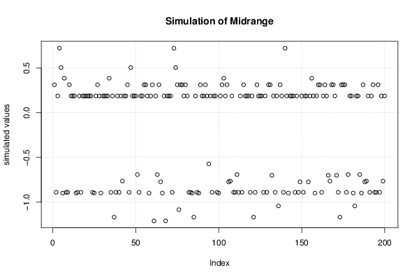
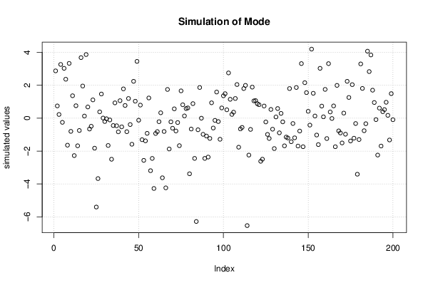
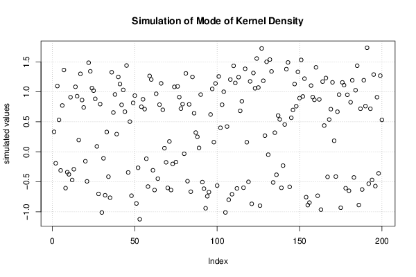
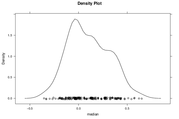
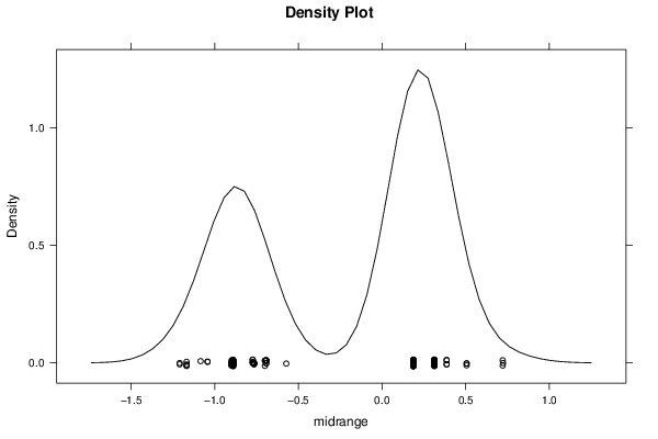
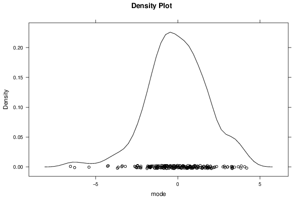
Title produced by software

Bootstrap Plot - Central Tendency

Date of computation

Sat, 13 Dec 2014 12:30:20 +0000

Cite this page as follows

Statistical Computations at FreeStatistics.org, Office for Research Development and Education, URL https://freestatistics.org/blog/index.php?v=date/2014/Dec/13/t1418473911qqam1kjq66o6pf0.htm/, Retrieved Thu, 16 May 2024 21:20:37 +0000

Statistical Computations at FreeStatistics.org, Office for Research Development and Education, URL https://freestatistics.org/blog/index.php?pk=267032, Retrieved Thu, 16 May 2024 21:20:37 +0000

QR Codes:

Paste this QR Code to cite your computation.

Original text written by user:

IsPrivate?

No (this computation is public)

User-defined keywords

Estimated Impact

106

Family? (F = Feedback message, R = changed R code, M = changed R Module, P = changed Parameters, D = changed Data)

-     [Bootstrap Plot - Central Tendency] [] [2014-11-04 10:49:59] [32b17a345b130fdf5cc88718ed94a974]
- R  D  [Bootstrap Plot - Central Tendency] [] [2014-11-12 15:33:27] [d253a55552bf9917a397def3be261e30]
-    D      [Bootstrap Plot - Central Tendency] [] [2014-12-13 12:30:20] [940a3d9bc049bdd1effc6e8b1116301d] [Current]
-    D        [Bootstrap Plot - Central Tendency] [] [2014-12-14 13:00:35] [d253a55552bf9917a397def3be261e30] 

Feedback Forum

Post a new message

Dataseries X:

Download CSV

Histogram

Boxplots

0.932222
-3.40718
2.02093
1.36824
-3.79056
-3.38055
-1.23504
3.31485
3.26324
-0.162007
-4.14466
-0.0353275
-5.40106
1.74394
-0.982709
-0.310041
1.91354
-0.325889
-0.891366
-2.14726
0.791716
-3.57529
2.88177
-2.73686
1.69897
0.900939
-3.62329
2.53661
3.31244
-0.603295
0.719479
-0.824002
0.425903
-4.314
-0.827149
-2.52479
1.55106
0.928113
-0.028673
1.74671
-2.28063
-0.527203
-3.45186
-0.169304
1.7191
-0.439106
3.83894
-1.61396
2.23742
-2.01029
4.19365
2.82941
0.87747
-1.05408
0.0306141
0.297232
2.82935
0.130906
-5.45826
4.74926
0.387721
2.65825
-2.69075
1.48456
-0.599803
2.58118
-2.44582
0.583253
-1.7366
-0.931429
2.46733
1.39476
-0.71745
1.43063
-0.856571
3.77843
-4.06047
1.74959
0.903734
1.95243
0.783888
0.324938
-1.66152
0.120254
3.16781
0.392802
-4.71512
-0.763504
1.02922
1.99095
2.11744
-1.09754
2.04121
3.91196
-4.33172
-1.18583
-1.20406
-2.32271
-1.32617
-3.74664
2.09148
3.67782
-2.24472
1.88483
-0.00112466
-0.559093
-1.10596
4.06807
-1.51748
3.86307
-4.82211
-1.81613
-0.670688
0.986877
1.79823
-6.13285
0.572984
3.02791
2.36338
-1.29867
1.30845
-3.13411
1.86285
-2.27486
2.066
1.25583
4.73285
-3.2583
-0.604271
1.2631
-2.04116
1.74526
1.25777
1.72918
-1.84841
1.11176
0.923519
0.269473
-0.636317
3.25515
-1.69528
1.4904
0.0861235
-0.204194
3.294
0.79281
2.87255
0.860894
0.265504
1.31237
-0.224824
-2.44669
0.15643
-1.19531
1.80645
-5.89349
1.35698
2.23385
-0.779467
1.36121
-0.612783
1.7998
1.09944
-2.84872
-2.49653
2.2386
0.508086
0.281476
6.90427
1.28433
-0.267105
1.46841
1.88506
-1.00054
-3.13529
0.778232
2.60497
-1.46431
-0.616958
-0.567452
2.72638
-0.932362
2.23324
-0.847608
-3.67248
-2.27175
-2.0986
2.3869
-0.0399423
-1.94751
0.437445
2.793
-1.84805
-1.67959
-0.145587
-2.57096
1.47757
-2.89814
3.2941
-0.537296
0.416
-2.11153
-0.190319
1.21825
0.950062
0.673744
0.372071
-1.07387
-0.478571
-0.12629
1.35631
-1.43241
0.440395
-0.797422
2.43008
1.65594
-0.383124
0.78967
-2.58556
-1.38788
-0.684021
-0.616442
1.34645
-1.24077
2.22666
-1.37847
-1.20355
1.99146
-4.27317
-0.773728
3.03373
2.60617
2.86588
2.76515
1.65633
3.63065
3.32698
3.51234
2.29815
-0.0894453
-2.15762
-2.02724
-6.27872
0.135422
-1.42627
-1.04298
-0.625054
-1.15017
-2.18658
0.754245
1.95562
4.1108
-2.5743
-1.1334
0.565461
0.942532
0.934201
-0.33767
-1.97428
-1.62172
-0.13279
1.19369
-1.64225
0.201401
-4.23566
-5.46212
-1.82565
-6.5295
-0.932446
-1.84111
-3.74594
1.18795
1.21946
-0.0542749
-0.669771
1.62901
2.03339
-1.02664
0.854178
-0.661109
0.620873
0.938601
0.513566
0.00438837
0.732725
-2.63675

Summary of computational transaction
Raw Input	view raw input (R code)
Raw Output	view raw output of R engine
Computing time	11 seconds
R Server	'Sir Ronald Aylmer Fisher' @ fisher.wessa.net

\begin{tabular}{lllllllll}
\hline
Summary of computational transaction \tabularnewline
Raw Input & view raw input (R code)  \tabularnewline
Raw Output & view raw output of R engine  \tabularnewline
Computing time & 11 seconds \tabularnewline
R Server & 'Sir Ronald Aylmer Fisher' @ fisher.wessa.net \tabularnewline
\hline
\end{tabular}
%Source: https://freestatistics.org/blog/index.php?pk=267032&T=0

[TABLE]
[ROW][C]Summary of computational transaction[/C][/ROW]
[ROW][C]Raw Input[/C][C]view raw input (R code) [/C][/ROW]
[ROW][C]Raw Output[/C][C]view raw output of R engine [/C][/ROW]
[ROW][C]Computing time[/C][C]11 seconds[/C][/ROW]
[ROW][C]R Server[/C][C]'Sir Ronald Aylmer Fisher' @ fisher.wessa.net[/C][/ROW]
[/TABLE]
Source: https://freestatistics.org/blog/index.php?pk=267032&T=0

Globally Unique Identifier (entire table): ba.freestatistics.org/blog/index.php?pk=267032&T=0

As an alternative you can also use a QR Code:

The GUIDs for individual cells are displayed in the table below:

Summary of computational transaction
Raw Input	view raw input (R code)
Raw Output	view raw output of R engine
Computing time	11 seconds
R Server	'Sir Ronald Aylmer Fisher' @ fisher.wessa.net

Estimation Results of Bootstrap
statistic	P1	P5	Q1	Estimate	Q3	P95	P99	S.D.	IQR
mean	-0.30186	-0.21795	-0.11268	5.3531e-08	0.093135	0.24106	0.32236	0.14716	0.20581
median	-0.33178	-0.19067	-0.038212	0.10319	0.27547	0.43315	0.57482	0.20986	0.31369
midrange	-1.1683	-0.89832	-0.89012	0.18739	0.18739	0.31642	0.72108	0.56311	1.0775
mode	-5.4098	-2.6498	-1.1615	5.3531e-08	1.0764	3.2648	3.8651	1.8329	2.2379
mode k.dens	-1.0103	-0.86136	-0.41316	0.42672	1.0827	1.4335	1.5566	0.78305	1.4958

\begin{tabular}{lllllllll}
\hline
Estimation Results of Bootstrap \tabularnewline
statistic & P1 & P5 & Q1 & Estimate & Q3 & P95 & P99 & S.D. & IQR \tabularnewline
mean & -0.30186 & -0.21795 & -0.11268 & 5.3531e-08 & 0.093135 & 0.24106 & 0.32236 & 0.14716 & 0.20581 \tabularnewline
median & -0.33178 & -0.19067 & -0.038212 & 0.10319 & 0.27547 & 0.43315 & 0.57482 & 0.20986 & 0.31369 \tabularnewline
midrange & -1.1683 & -0.89832 & -0.89012 & 0.18739 & 0.18739 & 0.31642 & 0.72108 & 0.56311 & 1.0775 \tabularnewline
mode & -5.4098 & -2.6498 & -1.1615 & 5.3531e-08 & 1.0764 & 3.2648 & 3.8651 & 1.8329 & 2.2379 \tabularnewline
mode k.dens & -1.0103 & -0.86136 & -0.41316 & 0.42672 & 1.0827 & 1.4335 & 1.5566 & 0.78305 & 1.4958 \tabularnewline
\hline
\end{tabular}
%Source: https://freestatistics.org/blog/index.php?pk=267032&T=1

[TABLE]
[ROW][C]Estimation Results of Bootstrap[/C][/ROW]
[ROW][C]statistic[/C][C]P1[/C][C]P5[/C][C]Q1[/C][C]Estimate[/C][C]Q3[/C][C]P95[/C][C]P99[/C][C]S.D.[/C][C]IQR[/C][/ROW]
[ROW][C]mean[/C][C]-0.30186[/C][C]-0.21795[/C][C]-0.11268[/C][C]5.3531e-08[/C][C]0.093135[/C][C]0.24106[/C][C]0.32236[/C][C]0.14716[/C][C]0.20581[/C][/ROW]
[ROW][C]median[/C][C]-0.33178[/C][C]-0.19067[/C][C]-0.038212[/C][C]0.10319[/C][C]0.27547[/C][C]0.43315[/C][C]0.57482[/C][C]0.20986[/C][C]0.31369[/C][/ROW]
[ROW][C]midrange[/C][C]-1.1683[/C][C]-0.89832[/C][C]-0.89012[/C][C]0.18739[/C][C]0.18739[/C][C]0.31642[/C][C]0.72108[/C][C]0.56311[/C][C]1.0775[/C][/ROW]
[ROW][C]mode[/C][C]-5.4098[/C][C]-2.6498[/C][C]-1.1615[/C][C]5.3531e-08[/C][C]1.0764[/C][C]3.2648[/C][C]3.8651[/C][C]1.8329[/C][C]2.2379[/C][/ROW]
[ROW][C]mode k.dens[/C][C]-1.0103[/C][C]-0.86136[/C][C]-0.41316[/C][C]0.42672[/C][C]1.0827[/C][C]1.4335[/C][C]1.5566[/C][C]0.78305[/C][C]1.4958[/C][/ROW]
[/TABLE]
Source: https://freestatistics.org/blog/index.php?pk=267032&T=1

Globally Unique Identifier (entire table): ba.freestatistics.org/blog/index.php?pk=267032&T=1

As an alternative you can also use a QR Code:

The GUIDs for individual cells are displayed in the table below:

Estimation Results of Bootstrap
statistic	P1	P5	Q1	Estimate	Q3	P95	P99	S.D.	IQR
mean	-0.30186	-0.21795	-0.11268	5.3531e-08	0.093135	0.24106	0.32236	0.14716	0.20581
median	-0.33178	-0.19067	-0.038212	0.10319	0.27547	0.43315	0.57482	0.20986	0.31369
midrange	-1.1683	-0.89832	-0.89012	0.18739	0.18739	0.31642	0.72108	0.56311	1.0775
mode	-5.4098	-2.6498	-1.1615	5.3531e-08	1.0764	3.2648	3.8651	1.8329	2.2379
mode k.dens	-1.0103	-0.86136	-0.41316	0.42672	1.0827	1.4335	1.5566	0.78305	1.4958

Figure 1

PNG link

Postscript link

PDF link

Figure 2

PNG link

Postscript link

PDF link

Figure 3

PNG link

Postscript link

PDF link

Figure 4

PNG link

Postscript link

PDF link

Figure 5

PNG link

Postscript link

PDF link

Figure 6

PNG link

Postscript link

PDF link

Figure 7

PNG link

Postscript link

PDF link

Figure 8

PNG link

Postscript link

PDF link

Figure 9

PNG link

Postscript link

PDF link

Figure 10

PNG link

Postscript link

PDF link

Figure 11

PNG link

Postscript link

PDF link

Parameters (Session):

par1 = 200 ; par2 = 5 ; par3 = 0 ; par4 = P1 P5 Q1 Q3 P95 P99 ;

Parameters (R input):

par1 = 200 ; par2 = 5 ; par3 = 0 ; par4 = P1 P5 Q1 Q3 P95 P99 ;

R code (references can be found in the software module):

par1 <- as.numeric(par1)
par2 <- as.numeric(par2)
if (par3 == '0') bw <- NULL
if (par3 != '0') bw <- as.numeric(par3)
if (par1 < 10) par1 = 10
if (par1 > 5000) par1 = 5000
library(modeest)
library(lattice)
library(boot)
boot.stat <- function(s,i)
{
s.mean <- mean(s[i])
s.median <- median(s[i])
s.midrange <- (max(s[i]) + min(s[i])) / 2
s.mode <- mlv(s[i], method='mfv')$M
s.kernelmode <- mlv(s[i], method='kernel', bw=bw)$M
c(s.mean, s.median, s.midrange, s.mode, s.kernelmode)
}
(r <- boot(x,boot.stat, R=par1, stype='i'))
bitmap(file='plot1.png')
plot(r$t[,1],type='p',ylab='simulated values',main='Simulation of Mean')
grid()
dev.off()
bitmap(file='plot2.png')
plot(r$t[,2],type='p',ylab='simulated values',main='Simulation of Median')
grid()
dev.off()
bitmap(file='plot3.png')
plot(r$t[,3],type='p',ylab='simulated values',main='Simulation of Midrange')
grid()
dev.off()
bitmap(file='plot7.png')
plot(r$t[,4],type='p',ylab='simulated values',main='Simulation of Mode')
grid()
dev.off()
bitmap(file='plot8.png')
plot(r$t[,5],type='p',ylab='simulated values',main='Simulation of Mode of Kernel Density')
grid()
dev.off()
bitmap(file='plot4.png')
densityplot(~r$t[,1],col='black',main='Density Plot',xlab='mean')
dev.off()
bitmap(file='plot5.png')
densityplot(~r$t[,2],col='black',main='Density Plot',xlab='median')
dev.off()
bitmap(file='plot6.png')
densityplot(~r$t[,3],col='black',main='Density Plot',xlab='midrange')
dev.off()
bitmap(file='plot9.png')
densityplot(~r$t[,4],col='black',main='Density Plot',xlab='mode')
dev.off()
bitmap(file='plot10.png')
densityplot(~r$t[,5],col='black',main='Density Plot',xlab='mode of kernel dens.')
dev.off()
z <- data.frame(cbind(r$t[,1],r$t[,2],r$t[,3],r$t[,4],r$t[,5]))
colnames(z) <- list('mean','median','midrange','mode','mode k.dens')
bitmap(file='plot11.png')
boxplot(z,notch=TRUE,ylab='simulated values',main='Bootstrap Simulation - Central Tendency')
grid()
dev.off()
load(file='createtable')
a<-table.start()
a<-table.row.start(a)
a<-table.element(a,'Estimation Results of Bootstrap',10,TRUE)
a<-table.row.end(a)
if (par4 == 'P1 P5 Q1 Q3 P95 P99') {
myq.1 <- 0.01
myq.2 <- 0.05
myq.3 <- 0.95
myq.4 <- 0.99
myl.1 <- 'P1'
myl.2 <- 'P5'
myl.3 <- 'P95'
myl.4 <- 'P99'
}
if (par4 == 'P0.5 P2.5 Q1 Q3 P97.5 P99.5') {
myq.1 <- 0.005
myq.2 <- 0.025
myq.3 <- 0.975
myq.4 <- 0.995
myl.1 <- 'P0.5'
myl.2 <- 'P2.5'
myl.3 <- 'P97.5'
myl.4 <- 'P99.5'
}
if (par4 == 'P10 P20 Q1 Q3 P80 P90') {
myq.1 <- 0.10
myq.2 <- 0.20
myq.3 <- 0.80
myq.4 <- 0.90
myl.1 <- 'P10'
myl.2 <- 'P20'
myl.3 <- 'P80'
myl.4 <- 'P90'
}
a<-table.row.start(a)
a<-table.element(a,'statistic',header=TRUE)
a<-table.element(a,myl.1,header=TRUE)
a<-table.element(a,myl.2,header=TRUE)
a<-table.element(a,'Q1',header=TRUE)
a<-table.element(a,'Estimate',header=TRUE)
a<-table.element(a,'Q3',header=TRUE)
a<-table.element(a,myl.3,header=TRUE)
a<-table.element(a,myl.4,header=TRUE)
a<-table.element(a,'S.D.',header=TRUE)
a<-table.element(a,'IQR',header=TRUE)
a<-table.row.end(a)
a<-table.row.start(a)
a<-table.element(a,'mean',header=TRUE)
q1 <- quantile(r$t[,1],0.25)[[1]]
q3 <- quantile(r$t[,1],0.75)[[1]]
p01 <- quantile(r$t[,1],myq.1)[[1]]
p05 <- quantile(r$t[,1],myq.2)[[1]]
p95 <- quantile(r$t[,1],myq.3)[[1]]
p99 <- quantile(r$t[,1],myq.4)[[1]]
a<-table.element(a,signif(p01,par2))
a<-table.element(a,signif(p05,par2))
a<-table.element(a,signif(q1,par2))
a<-table.element(a,signif(r$t0[1],par2))
a<-table.element(a,signif(q3,par2))
a<-table.element(a,signif(p95,par2))
a<-table.element(a,signif(p99,par2))
a<-table.element( a,signif( sqrt(var(r$t[,1])),par2 ) )
a<-table.element(a,signif(q3-q1,par2))
a<-table.row.end(a)
a<-table.row.start(a)
a<-table.element(a,'median',header=TRUE)
q1 <- quantile(r$t[,2],0.25)[[1]]
q3 <- quantile(r$t[,2],0.75)[[1]]
p01 <- quantile(r$t[,2],myq.1)[[1]]
p05 <- quantile(r$t[,2],myq.2)[[1]]
p95 <- quantile(r$t[,2],myq.3)[[1]]
p99 <- quantile(r$t[,2],myq.4)[[1]]
a<-table.element(a,signif(p01,par2))
a<-table.element(a,signif(p05,par2))
a<-table.element(a,signif(q1,par2))
a<-table.element(a,signif(r$t0[2],par2))
a<-table.element(a,signif(q3,par2))
a<-table.element(a,signif(p95,par2))
a<-table.element(a,signif(p99,par2))
a<-table.element(a,signif(sqrt(var(r$t[,2])),par2))
a<-table.element(a,signif(q3-q1,par2))
a<-table.row.end(a)
a<-table.row.start(a)
a<-table.element(a,'midrange',header=TRUE)
q1 <- quantile(r$t[,3],0.25)[[1]]
q3 <- quantile(r$t[,3],0.75)[[1]]
p01 <- quantile(r$t[,3],myq.1)[[1]]
p05 <- quantile(r$t[,3],myq.2)[[1]]
p95 <- quantile(r$t[,3],myq.3)[[1]]
p99 <- quantile(r$t[,3],myq.4)[[1]]
a<-table.element(a,signif(p01,par2))
a<-table.element(a,signif(p05,par2))
a<-table.element(a,signif(q1,par2))
a<-table.element(a,signif(r$t0[3],par2))
a<-table.element(a,signif(q3,par2))
a<-table.element(a,signif(p95,par2))
a<-table.element(a,signif(p99,par2))
a<-table.element(a,signif(sqrt(var(r$t[,3])),par2))
a<-table.element(a,signif(q3-q1,par2))
a<-table.row.end(a)
a<-table.row.start(a)
a<-table.element(a,'mode',header=TRUE)
q1 <- quantile(r$t[,4],0.25)[[1]]
q3 <- quantile(r$t[,4],0.75)[[1]]
p01 <- quantile(r$t[,4],myq.1)[[1]]
p05 <- quantile(r$t[,4],myq.2)[[1]]
p95 <- quantile(r$t[,4],myq.3)[[1]]
p99 <- quantile(r$t[,4],myq.4)[[1]]
a<-table.element(a,signif(p01,par2))
a<-table.element(a,signif(p05,par2))
a<-table.element(a,signif(q1,par2))
a<-table.element(a,signif(r$t0[4],par2))
a<-table.element(a,signif(q3,par2))
a<-table.element(a,signif(p95,par2))
a<-table.element(a,signif(p99,par2))
a<-table.element(a,signif(sqrt(var(r$t[,4])),par2))
a<-table.element(a,signif(q3-q1,par2))
a<-table.row.end(a)
a<-table.row.start(a)
a<-table.element(a,'mode k.dens',header=TRUE)
q1 <- quantile(r$t[,5],0.25)[[1]]
q3 <- quantile(r$t[,5],0.75)[[1]]
p01 <- quantile(r$t[,5],myq.1)[[1]]
p05 <- quantile(r$t[,5],myq.2)[[1]]
p95 <- quantile(r$t[,5],myq.3)[[1]]
p99 <- quantile(r$t[,5],myq.4)[[1]]
a<-table.element(a,signif(p01,par2))
a<-table.element(a,signif(p05,par2))
a<-table.element(a,signif(q1,par2))
a<-table.element(a,signif(r$t0[5],par2))
a<-table.element(a,signif(q3,par2))
a<-table.element(a,signif(p95,par2))
a<-table.element(a,signif(p99,par2))
a<-table.element(a,signif(sqrt(var(r$t[,5])),par2))
a<-table.element(a,signif(q3-q1,par2))
a<-table.row.end(a)
a<-table.end(a)
table.save(a,file='mytable.tab')

Free Statistics

Description of Statistical Computation

Tree of Dependent Computations

Dataset

Tables (Output of Computation)

Figures (Output of Computation)

Input Parameters & R Code