Free Statistics
of Irreproducible Research!
Description of Statistical Computation | |||||||||||||||||||||||||||||||||||||||||||||||||||||||||||||||||||||||||||||||||||||||||||||||||||||||||||||
|---|---|---|---|---|---|---|---|---|---|---|---|---|---|---|---|---|---|---|---|---|---|---|---|---|---|---|---|---|---|---|---|---|---|---|---|---|---|---|---|---|---|---|---|---|---|---|---|---|---|---|---|---|---|---|---|---|---|---|---|---|---|---|---|---|---|---|---|---|---|---|---|---|---|---|---|---|---|---|---|---|---|---|---|---|---|---|---|---|---|---|---|---|---|---|---|---|---|---|---|---|---|---|---|---|---|---|---|---|---|
| Author's title | |||||||||||||||||||||||||||||||||||||||||||||||||||||||||||||||||||||||||||||||||||||||||||||||||||||||||||||
| Author | *The author of this computation has been verified* | ||||||||||||||||||||||||||||||||||||||||||||||||||||||||||||||||||||||||||||||||||||||||||||||||||||||||||||
| R Software Module | rwasp_correlation.wasp | ||||||||||||||||||||||||||||||||||||||||||||||||||||||||||||||||||||||||||||||||||||||||||||||||||||||||||||
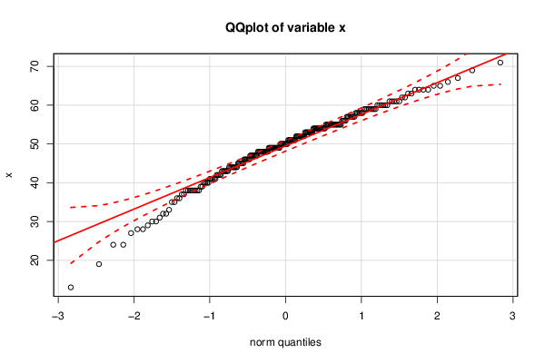
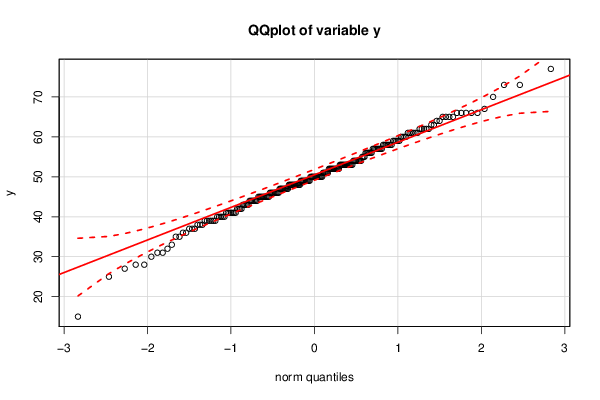
| Title produced by software | Pearson Correlation | ||||||||||||||||||||||||||||||||||||||||||||||||||||||||||||||||||||||||||||||||||||||||||||||||||||||||||||
| Date of computation | Sat, 13 Dec 2014 15:36:00 +0000 | ||||||||||||||||||||||||||||||||||||||||||||||||||||||||||||||||||||||||||||||||||||||||||||||||||||||||||||
| Cite this page as follows | Statistical Computations at FreeStatistics.org, Office for Research Development and Education, URL https://freestatistics.org/blog/index.php?v=date/2014/Dec/13/t1418485019huqsvnazji8nw2m.htm/, Retrieved Thu, 16 May 2024 17:35:06 +0000 | ||||||||||||||||||||||||||||||||||||||||||||||||||||||||||||||||||||||||||||||||||||||||||||||||||||||||||||
| Statistical Computations at FreeStatistics.org, Office for Research Development and Education, URL https://freestatistics.org/blog/index.php?pk=267163, Retrieved Thu, 16 May 2024 17:35:06 +0000 | |||||||||||||||||||||||||||||||||||||||||||||||||||||||||||||||||||||||||||||||||||||||||||||||||||||||||||||
| QR Codes: | |||||||||||||||||||||||||||||||||||||||||||||||||||||||||||||||||||||||||||||||||||||||||||||||||||||||||||||
|
| |||||||||||||||||||||||||||||||||||||||||||||||||||||||||||||||||||||||||||||||||||||||||||||||||||||||||||||
| Original text written by user: | |||||||||||||||||||||||||||||||||||||||||||||||||||||||||||||||||||||||||||||||||||||||||||||||||||||||||||||
| IsPrivate? | No (this computation is public) | ||||||||||||||||||||||||||||||||||||||||||||||||||||||||||||||||||||||||||||||||||||||||||||||||||||||||||||
| User-defined keywords | |||||||||||||||||||||||||||||||||||||||||||||||||||||||||||||||||||||||||||||||||||||||||||||||||||||||||||||
| Estimated Impact | 102 | ||||||||||||||||||||||||||||||||||||||||||||||||||||||||||||||||||||||||||||||||||||||||||||||||||||||||||||
Tree of Dependent Computations | |||||||||||||||||||||||||||||||||||||||||||||||||||||||||||||||||||||||||||||||||||||||||||||||||||||||||||||
| Family? (F = Feedback message, R = changed R code, M = changed R Module, P = changed Parameters, D = changed Data) | |||||||||||||||||||||||||||||||||||||||||||||||||||||||||||||||||||||||||||||||||||||||||||||||||||||||||||||
| - [Percentiles] [Intrinsic Motivat...] [2010-10-12 12:10:58] [b98453cac15ba1066b407e146608df68] - RMPD [Kernel Density Estimation] [] [2011-10-18 22:42:23] [b98453cac15ba1066b407e146608df68] - RMPD [Percentiles] [] [2011-10-18 22:46:45] [b98453cac15ba1066b407e146608df68] - RMPD [Notched Boxplots] [] [2011-10-18 22:58:56] [b98453cac15ba1066b407e146608df68] - RM D [Back to Back Histogram] [] [2011-10-18 23:05:48] [b98453cac15ba1066b407e146608df68] - RMPD [Pearson Correlation] [WS3: question 4 (...] [2014-10-16 20:35:26] [1764622206627ac897c737076a0cb4c8] - D [Pearson Correlation] [] [2014-12-13 15:36:00] [6260c34aa94cecca073345f42e0d4b5d] [Current] | |||||||||||||||||||||||||||||||||||||||||||||||||||||||||||||||||||||||||||||||||||||||||||||||||||||||||||||
| Feedback Forum | |||||||||||||||||||||||||||||||||||||||||||||||||||||||||||||||||||||||||||||||||||||||||||||||||||||||||||||
Post a new message | |||||||||||||||||||||||||||||||||||||||||||||||||||||||||||||||||||||||||||||||||||||||||||||||||||||||||||||
Dataset | |||||||||||||||||||||||||||||||||||||||||||||||||||||||||||||||||||||||||||||||||||||||||||||||||||||||||||||
| Dataseries X: | |||||||||||||||||||||||||||||||||||||||||||||||||||||||||||||||||||||||||||||||||||||||||||||||||||||||||||||
24 47 36 47 55 66 57 52 67 54 46 49 28 50 52 45 64 63 39 42 54 36 49 60 33 46 48 52 35 40 63 32 45 51 48 38 59 53 50 30 61 61 47 51 44 54 53 58 49 53 48 40 55 55 52 50 37 47 51 45 57 28 53 60 38 44 40 48 48 62 58 47 24 41 47 37 54 53 55 57 58 58 35 43 44 45 61 53 41 38 41 55 51 54 39 48 54 59 47 44 55 48 59 48 51 65 46 44 38 58 50 19 54 60 50 50 48 32 69 55 52 53 41 53 56 55 13 52 46 56 27 53 45 52 31 38 41 44 49 51 40 49 51 43 56 38 42 55 55 44 49 51 42 57 43 48 59 55 50 30 54 49 48 59 43 49 56 49 50 49 29 44 57 57 49 54 60 58 62 43 54 49 64 55 54 64 45 59 50 57 65 60 55 46 61 43 55 47 38 59 48 51 55 71 54 60 42 49 52 61 52 52 54 38 64 46 59 | |||||||||||||||||||||||||||||||||||||||||||||||||||||||||||||||||||||||||||||||||||||||||||||||||||||||||||||
| Dataseries Y: | |||||||||||||||||||||||||||||||||||||||||||||||||||||||||||||||||||||||||||||||||||||||||||||||||||||||||||||
52 62 40 48 40 77 61 44 66 49 40 53 59 58 53 58 49 51 58 48 53 39 47 51 52 57 37 46 48 33 28 45 56 45 53 47 39 62 59 55 50 45 59 39 41 53 44 61 41 54 36 47 54 54 57 47 32 66 41 54 54 40 60 53 25 58 50 56 48 15 43 52 49 46 56 62 48 50 35 50 67 48 42 48 58 31 60 43 50 57 30 44 65 49 70 48 54 52 61 61 66 53 56 44 50 73 52 53 53 48 45 44 50 31 50 43 64 56 46 41 58 46 52 37 50 46 51 54 47 35 57 44 49 45 57 58 63 46 52 53 57 27 59 52 51 45 53 38 60 51 45 39 52 39 48 38 57 47 62 57 45 55 43 53 51 28 41 49 50 42 40 41 42 46 49 52 54 50 61 52 49 39 61 41 63 62 46 47 65 44 37 66 73 38 49 64 56 42 36 45 45 47 59 48 53 50 49 65 47 60 46 50 55 48 43 66 65 52 38 44 61 41 38 64 59 54 36 34 48 55 44 46 53 20 49 35 62 41 36 54 59 54 54 52 39 50 59 53 43 55 56 45 42 42 53 51 38 51 61 57 55 62 23 52 48 55 43 44 70 31 45 49 66 49 46 50 48 58 62 55 49 | |||||||||||||||||||||||||||||||||||||||||||||||||||||||||||||||||||||||||||||||||||||||||||||||||||||||||||||
Tables (Output of Computation) | |||||||||||||||||||||||||||||||||||||||||||||||||||||||||||||||||||||||||||||||||||||||||||||||||||||||||||||
| |||||||||||||||||||||||||||||||||||||||||||||||||||||||||||||||||||||||||||||||||||||||||||||||||||||||||||||
Figures (Output of Computation) | |||||||||||||||||||||||||||||||||||||||||||||||||||||||||||||||||||||||||||||||||||||||||||||||||||||||||||||
Input Parameters & R Code | |||||||||||||||||||||||||||||||||||||||||||||||||||||||||||||||||||||||||||||||||||||||||||||||||||||||||||||
| Parameters (Session): | |||||||||||||||||||||||||||||||||||||||||||||||||||||||||||||||||||||||||||||||||||||||||||||||||||||||||||||
| Parameters (R input): | |||||||||||||||||||||||||||||||||||||||||||||||||||||||||||||||||||||||||||||||||||||||||||||||||||||||||||||
| R code (references can be found in the software module): | |||||||||||||||||||||||||||||||||||||||||||||||||||||||||||||||||||||||||||||||||||||||||||||||||||||||||||||
x <- x[!is.na(y)] | |||||||||||||||||||||||||||||||||||||||||||||||||||||||||||||||||||||||||||||||||||||||||||||||||||||||||||||