Free Statistics
of Irreproducible Research!
Description of Statistical Computation | |||||||||||||||||||||||||||||||||||||||||||||||||||||||||||||||||||||||||||||||||||||||||||||||||||||||||||||
|---|---|---|---|---|---|---|---|---|---|---|---|---|---|---|---|---|---|---|---|---|---|---|---|---|---|---|---|---|---|---|---|---|---|---|---|---|---|---|---|---|---|---|---|---|---|---|---|---|---|---|---|---|---|---|---|---|---|---|---|---|---|---|---|---|---|---|---|---|---|---|---|---|---|---|---|---|---|---|---|---|---|---|---|---|---|---|---|---|---|---|---|---|---|---|---|---|---|---|---|---|---|---|---|---|---|---|---|---|---|
| Author's title | |||||||||||||||||||||||||||||||||||||||||||||||||||||||||||||||||||||||||||||||||||||||||||||||||||||||||||||
| Author | *The author of this computation has been verified* | ||||||||||||||||||||||||||||||||||||||||||||||||||||||||||||||||||||||||||||||||||||||||||||||||||||||||||||
| R Software Module | rwasp_correlation.wasp | ||||||||||||||||||||||||||||||||||||||||||||||||||||||||||||||||||||||||||||||||||||||||||||||||||||||||||||
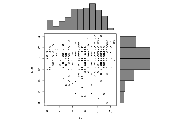
| Title produced by software | Pearson Correlation | ||||||||||||||||||||||||||||||||||||||||||||||||||||||||||||||||||||||||||||||||||||||||||||||||||||||||||||
| Date of computation | Sun, 14 Dec 2014 11:31:07 +0000 | ||||||||||||||||||||||||||||||||||||||||||||||||||||||||||||||||||||||||||||||||||||||||||||||||||||||||||||
| Cite this page as follows | Statistical Computations at FreeStatistics.org, Office for Research Development and Education, URL https://freestatistics.org/blog/index.php?v=date/2014/Dec/14/t1418556875x4cjuxa4ye77geq.htm/, Retrieved Thu, 16 May 2024 12:57:02 +0000 | ||||||||||||||||||||||||||||||||||||||||||||||||||||||||||||||||||||||||||||||||||||||||||||||||||||||||||||
| Statistical Computations at FreeStatistics.org, Office for Research Development and Education, URL https://freestatistics.org/blog/index.php?pk=267455, Retrieved Thu, 16 May 2024 12:57:02 +0000 | |||||||||||||||||||||||||||||||||||||||||||||||||||||||||||||||||||||||||||||||||||||||||||||||||||||||||||||
| QR Codes: | |||||||||||||||||||||||||||||||||||||||||||||||||||||||||||||||||||||||||||||||||||||||||||||||||||||||||||||
|
| |||||||||||||||||||||||||||||||||||||||||||||||||||||||||||||||||||||||||||||||||||||||||||||||||||||||||||||
| Original text written by user: | |||||||||||||||||||||||||||||||||||||||||||||||||||||||||||||||||||||||||||||||||||||||||||||||||||||||||||||
| IsPrivate? | No (this computation is public) | ||||||||||||||||||||||||||||||||||||||||||||||||||||||||||||||||||||||||||||||||||||||||||||||||||||||||||||
| User-defined keywords | |||||||||||||||||||||||||||||||||||||||||||||||||||||||||||||||||||||||||||||||||||||||||||||||||||||||||||||
| Estimated Impact | 83 | ||||||||||||||||||||||||||||||||||||||||||||||||||||||||||||||||||||||||||||||||||||||||||||||||||||||||||||
Tree of Dependent Computations | |||||||||||||||||||||||||||||||||||||||||||||||||||||||||||||||||||||||||||||||||||||||||||||||||||||||||||||
| Family? (F = Feedback message, R = changed R code, M = changed R Module, P = changed Parameters, D = changed Data) | |||||||||||||||||||||||||||||||||||||||||||||||||||||||||||||||||||||||||||||||||||||||||||||||||||||||||||||
| - [Pearson Correlation] [] [2014-12-14 11:31:07] [6e98989d1e11d52934121e5a163a7817] [Current] | |||||||||||||||||||||||||||||||||||||||||||||||||||||||||||||||||||||||||||||||||||||||||||||||||||||||||||||
| Feedback Forum | |||||||||||||||||||||||||||||||||||||||||||||||||||||||||||||||||||||||||||||||||||||||||||||||||||||||||||||
Post a new message | |||||||||||||||||||||||||||||||||||||||||||||||||||||||||||||||||||||||||||||||||||||||||||||||||||||||||||||
Dataset | |||||||||||||||||||||||||||||||||||||||||||||||||||||||||||||||||||||||||||||||||||||||||||||||||||||||||||||
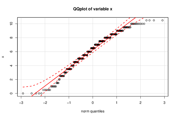
| Dataseries X: | |||||||||||||||||||||||||||||||||||||||||||||||||||||||||||||||||||||||||||||||||||||||||||||||||||||||||||||
7,5 2,5 6,0 6,5 1,0 1,0 5,5 8,5 6,5 4,5 2,0 5,0 0,5 5,0 5,0 2,5 5,0 5,5 3,5 3,0 4,0 0,5 6,5 4,5 7,5 5,5 4,0 7,5 7,0 4,0 5,5 2,5 5,5 0,5 3,5 2,5 4,5 4,5 4,5 6,0 2,5 5,0 0,0 5,0 6,5 5,0 6,0 4,5 5,5 1,0 7,5 6,0 5,0 1,0 5,0 6,5 7,0 4,5 0,0 8,5 3,5 7,5 3,5 6,0 1,5 9,0 3,5 3,5 4,0 6,5 7,5 6,0 5,0 5,5 3,5 7,5 1,0 6,5 NA 6,5 6,5 7,0 3,5 1,5 4,0 7,5 4,5 0,0 3,5 5,5 5,0 4,5 2,5 7,5 7,0 0,0 4,5 3,0 1,5 3,5 2,5 5,5 8,0 1,0 5,0 4,5 3,0 3,0 8,0 2,5 7,0 0,0 1,0 3,5 5,5 5,5 0,5 7,5 9 9,5 8,5 7 8 10 7 8,5 9 9,5 4 6 8 5,5 9,5 7,5 7 7,5 8 7 7 6 10 2,5 9 8 6 8,5 6 9 8 8 9 5,5 5 7 5,5 9 2 8,5 9 8,5 9 7,5 10 9 7,5 6 10,5 8,5 8 10 10,5 6,5 9,5 8,5 7,5 5 8 10 7 7,5 7,5 9,5 6 10 7 3 6 7 10 7 3,5 8 10 5,5 6 6,5 6,5 8,5 4 9,5 8 8,5 5,5 7 9 8 10 8 6 8 5 9 4,5 8,5 7 9,5 8,5 7,5 7,5 5 7 8 5,5 8,5 7,5 9,5 7 8 8,5 3,5 6,5 6,5 10,5 8,5 8 10 10 9,5 9 10 7,5 4,5 4,5 0,5 6,5 4,5 5,5 5 6 4 8 10,5 8,5 6,5 8 8,5 5,5 7 5 3,5 5 9 8,5 5 9,5 3 1,5 6 0,5 6,5 7,5 4,5 8 9 7,5 8,5 7 9,5 6,5 9,5 6 8 9,5 8 8 9 5 | |||||||||||||||||||||||||||||||||||||||||||||||||||||||||||||||||||||||||||||||||||||||||||||||||||||||||||||
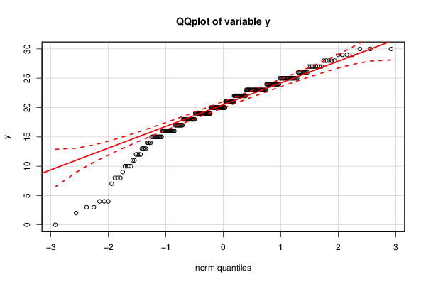
| Dataseries Y: | |||||||||||||||||||||||||||||||||||||||||||||||||||||||||||||||||||||||||||||||||||||||||||||||||||||||||||||
21 26 22 22 18 23 12 20 22 21 19 22 15 20 19 18 15 20 21 21 15 16 23 21 18 25 9 30 20 23 16 16 19 25 25 18 23 21 10 14 22 26 23 23 24 24 18 23 15 19 16 25 23 17 19 21 18 27 21 13 8 29 28 23 21 19 19 20 18 19 17 19 25 19 22 23 26 14 28 16 24 20 12 24 22 12 22 20 10 23 17 22 24 18 21 20 20 22 19 20 26 23 24 21 21 19 8 17 20 11 8 15 18 18 19 19 23 22 21 25 30 17 27 23 23 18 18 23 19 15 20 16 24 25 25 19 19 16 19 19 23 21 22 19 20 20 3 23 14 23 20 15 13 16 7 24 17 24 24 19 25 20 28 23 27 18 28 21 19 23 27 22 28 25 21 22 28 20 29 25 25 20 20 16 20 20 23 18 25 18 19 25 25 25 24 19 26 10 17 13 17 30 25 4 16 21 23 22 17 20 20 22 16 23 16 0 18 25 23 12 18 24 11 18 14 23 24 29 18 15 29 16 19 22 16 23 23 19 4 20 24 20 4 24 22 16 3 15 24 17 20 27 23 26 23 17 20 22 19 24 19 23 15 27 26 22 22 18 15 22 27 10 20 17 23 19 13 27 23 16 25 2 26 20 23 22 24 | |||||||||||||||||||||||||||||||||||||||||||||||||||||||||||||||||||||||||||||||||||||||||||||||||||||||||||||
Tables (Output of Computation) | |||||||||||||||||||||||||||||||||||||||||||||||||||||||||||||||||||||||||||||||||||||||||||||||||||||||||||||
| |||||||||||||||||||||||||||||||||||||||||||||||||||||||||||||||||||||||||||||||||||||||||||||||||||||||||||||
Figures (Output of Computation) | |||||||||||||||||||||||||||||||||||||||||||||||||||||||||||||||||||||||||||||||||||||||||||||||||||||||||||||
Input Parameters & R Code | |||||||||||||||||||||||||||||||||||||||||||||||||||||||||||||||||||||||||||||||||||||||||||||||||||||||||||||
| Parameters (Session): | |||||||||||||||||||||||||||||||||||||||||||||||||||||||||||||||||||||||||||||||||||||||||||||||||||||||||||||
| Parameters (R input): | |||||||||||||||||||||||||||||||||||||||||||||||||||||||||||||||||||||||||||||||||||||||||||||||||||||||||||||
| R code (references can be found in the software module): | |||||||||||||||||||||||||||||||||||||||||||||||||||||||||||||||||||||||||||||||||||||||||||||||||||||||||||||
x <- x[!is.na(y)] | |||||||||||||||||||||||||||||||||||||||||||||||||||||||||||||||||||||||||||||||||||||||||||||||||||||||||||||