Free Statistics
of Irreproducible Research!
Description of Statistical Computation | |||||||||||||||||||||||||||||||||||||||||||||||||||||||||||||||||||||||||||||||||||||||||||||||||||||||||||||||||||||||||||||||||||||||||||||||||||||||||||||||||
|---|---|---|---|---|---|---|---|---|---|---|---|---|---|---|---|---|---|---|---|---|---|---|---|---|---|---|---|---|---|---|---|---|---|---|---|---|---|---|---|---|---|---|---|---|---|---|---|---|---|---|---|---|---|---|---|---|---|---|---|---|---|---|---|---|---|---|---|---|---|---|---|---|---|---|---|---|---|---|---|---|---|---|---|---|---|---|---|---|---|---|---|---|---|---|---|---|---|---|---|---|---|---|---|---|---|---|---|---|---|---|---|---|---|---|---|---|---|---|---|---|---|---|---|---|---|---|---|---|---|---|---|---|---|---|---|---|---|---|---|---|---|---|---|---|---|---|---|---|---|---|---|---|---|---|---|---|---|---|---|---|---|
| Author's title | |||||||||||||||||||||||||||||||||||||||||||||||||||||||||||||||||||||||||||||||||||||||||||||||||||||||||||||||||||||||||||||||||||||||||||||||||||||||||||||||||
| Author | *The author of this computation has been verified* | ||||||||||||||||||||||||||||||||||||||||||||||||||||||||||||||||||||||||||||||||||||||||||||||||||||||||||||||||||||||||||||||||||||||||||||||||||||||||||||||||
| R Software Module | rwasp_bootstrapplot1.wasp | ||||||||||||||||||||||||||||||||||||||||||||||||||||||||||||||||||||||||||||||||||||||||||||||||||||||||||||||||||||||||||||||||||||||||||||||||||||||||||||||||
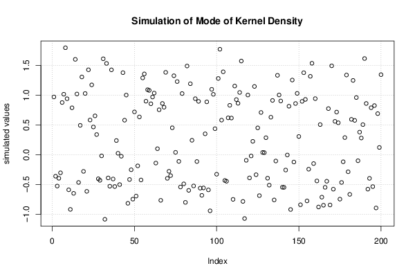
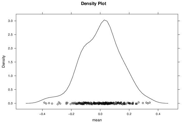
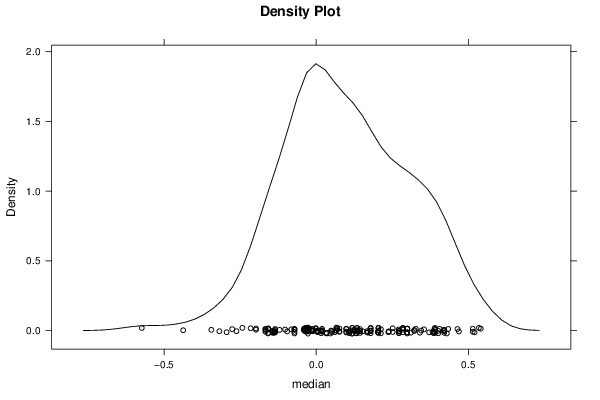
| Title produced by software | Bootstrap Plot - Central Tendency | ||||||||||||||||||||||||||||||||||||||||||||||||||||||||||||||||||||||||||||||||||||||||||||||||||||||||||||||||||||||||||||||||||||||||||||||||||||||||||||||||
| Date of computation | Sun, 14 Dec 2014 13:00:35 +0000 | ||||||||||||||||||||||||||||||||||||||||||||||||||||||||||||||||||||||||||||||||||||||||||||||||||||||||||||||||||||||||||||||||||||||||||||||||||||||||||||||||
| Cite this page as follows | Statistical Computations at FreeStatistics.org, Office for Research Development and Education, URL https://freestatistics.org/blog/index.php?v=date/2014/Dec/14/t1418562088eb0xss8gu4oogof.htm/, Retrieved Thu, 16 May 2024 06:29:19 +0000 | ||||||||||||||||||||||||||||||||||||||||||||||||||||||||||||||||||||||||||||||||||||||||||||||||||||||||||||||||||||||||||||||||||||||||||||||||||||||||||||||||
| Statistical Computations at FreeStatistics.org, Office for Research Development and Education, URL https://freestatistics.org/blog/index.php?pk=267532, Retrieved Thu, 16 May 2024 06:29:19 +0000 | |||||||||||||||||||||||||||||||||||||||||||||||||||||||||||||||||||||||||||||||||||||||||||||||||||||||||||||||||||||||||||||||||||||||||||||||||||||||||||||||||
| QR Codes: | |||||||||||||||||||||||||||||||||||||||||||||||||||||||||||||||||||||||||||||||||||||||||||||||||||||||||||||||||||||||||||||||||||||||||||||||||||||||||||||||||
|
| |||||||||||||||||||||||||||||||||||||||||||||||||||||||||||||||||||||||||||||||||||||||||||||||||||||||||||||||||||||||||||||||||||||||||||||||||||||||||||||||||
| Original text written by user: | |||||||||||||||||||||||||||||||||||||||||||||||||||||||||||||||||||||||||||||||||||||||||||||||||||||||||||||||||||||||||||||||||||||||||||||||||||||||||||||||||
| IsPrivate? | No (this computation is public) | ||||||||||||||||||||||||||||||||||||||||||||||||||||||||||||||||||||||||||||||||||||||||||||||||||||||||||||||||||||||||||||||||||||||||||||||||||||||||||||||||
| User-defined keywords | |||||||||||||||||||||||||||||||||||||||||||||||||||||||||||||||||||||||||||||||||||||||||||||||||||||||||||||||||||||||||||||||||||||||||||||||||||||||||||||||||
| Estimated Impact | 104 | ||||||||||||||||||||||||||||||||||||||||||||||||||||||||||||||||||||||||||||||||||||||||||||||||||||||||||||||||||||||||||||||||||||||||||||||||||||||||||||||||
Tree of Dependent Computations | |||||||||||||||||||||||||||||||||||||||||||||||||||||||||||||||||||||||||||||||||||||||||||||||||||||||||||||||||||||||||||||||||||||||||||||||||||||||||||||||||
| Family? (F = Feedback message, R = changed R code, M = changed R Module, P = changed Parameters, D = changed Data) | |||||||||||||||||||||||||||||||||||||||||||||||||||||||||||||||||||||||||||||||||||||||||||||||||||||||||||||||||||||||||||||||||||||||||||||||||||||||||||||||||
| - [Bootstrap Plot - Central Tendency] [] [2014-11-04 10:49:59] [32b17a345b130fdf5cc88718ed94a974] - R D [Bootstrap Plot - Central Tendency] [] [2014-11-12 15:33:27] [d253a55552bf9917a397def3be261e30] - D [Bootstrap Plot - Central Tendency] [] [2014-12-13 12:30:20] [d253a55552bf9917a397def3be261e30] - D [Bootstrap Plot - Central Tendency] [] [2014-12-14 13:00:35] [940a3d9bc049bdd1effc6e8b1116301d] [Current] | |||||||||||||||||||||||||||||||||||||||||||||||||||||||||||||||||||||||||||||||||||||||||||||||||||||||||||||||||||||||||||||||||||||||||||||||||||||||||||||||||
| Feedback Forum | |||||||||||||||||||||||||||||||||||||||||||||||||||||||||||||||||||||||||||||||||||||||||||||||||||||||||||||||||||||||||||||||||||||||||||||||||||||||||||||||||
Post a new message | |||||||||||||||||||||||||||||||||||||||||||||||||||||||||||||||||||||||||||||||||||||||||||||||||||||||||||||||||||||||||||||||||||||||||||||||||||||||||||||||||
Dataset | |||||||||||||||||||||||||||||||||||||||||||||||||||||||||||||||||||||||||||||||||||||||||||||||||||||||||||||||||||||||||||||||||||||||||||||||||||||||||||||||||
| Dataseries X: | |||||||||||||||||||||||||||||||||||||||||||||||||||||||||||||||||||||||||||||||||||||||||||||||||||||||||||||||||||||||||||||||||||||||||||||||||||||||||||||||||
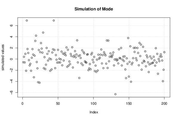
0.930232 -3.40521 2.02182 1.36969 -3.79215 -3.37923 -1.23382 3.31456 3.26075 -0.165989 -4.14243 -0.0335755 -5.40131 1.74607 -0.986595 -0.309542 1.91394 -0.327325 -0.89044 -2.14762 0.791583 -3.57304 2.88251 -2.73464 1.69646 0.902231 -3.62451 2.53148 3.31196 -0.604015 0.720093 -0.824376 0.429387 -4.31361 -0.823784 -2.52619 1.55265 0.929294 -0.0289107 1.74827 -2.28123 -0.525751 -3.45105 -0.167651 1.71842 -0.437273 3.83774 -1.61331 2.23669 -2.01368 4.19201 2.83074 0.877681 -1.05345 0.0338844 0.299579 2.82962 0.134707 -5.45701 4.75094 0.386812 2.65834 -2.6914 1.48738 -0.597236 2.58097 -2.44384 0.583801 -1.73785 -0.934774 2.46862 1.39291 -0.717696 1.43155 -0.856457 3.77396 -4.06016 1.74878 0.903159 1.95283 0.784645 0.322499 -1.6619 0.118537 3.16621 0.390905 -4.71432 -0.766198 1.02652 1.98851 2.11668 -1.09769 2.04049 3.91253 -4.32922 -1.18636 -1.20051 -2.32142 -1.32521 -3.74392 2.09449 3.67999 -2.24686 1.8847 -0.00138148 -0.561207 -1.10791 4.06735 -1.52051 3.86172 -4.82336 -1.81619 -0.673258 0.986615 1.79907 -6.14221 0.571834 3.01493 2.35191 -1.29061 1.30383 -3.13186 1.86218 -2.27961 2.06061 1.25248 4.74694 -3.25767 -0.605609 1.25981 -2.05434 1.74765 1.25994 1.73564 -1.85395 1.10537 0.938882 0.27089 -0.636737 3.25287 -1.69574 1.49124 0.0988109 -0.207916 3.28949 0.804418 2.87297 0.859365 0.272281 1.31216 -0.22338 -2.44715 0.153112 -1.1713 1.80552 -5.87528 1.33443 2.2369 -0.781063 1.36043 -0.629536 1.79828 1.09999 -2.85353 -2.49528 2.25146 0.520604 0.298607 6.90909 1.28231 -0.262004 1.46464 1.88438 -1.00143 -3.14066 0.777597 2.59824 -1.46655 -0.635298 -0.585772 2.72724 -0.934081 2.22985 -0.851462 -3.65571 -2.27573 -2.09533 2.38629 -0.0258131 -1.94653 0.438568 2.79009 -1.83582 -1.66756 -0.150236 -2.58702 1.49501 -2.89766 3.28964 -0.539803 0.420198 -2.1092 -0.188277 1.23821 0.941709 0.680047 0.382231 -1.0876 -0.493543 -0.135096 1.36667 -1.43758 0.420898 -0.779616 2.42003 1.67243 -0.386505 0.797683 -2.59059 -1.38176 -0.683298 -0.61428 1.34484 -1.2397 2.23363 -1.38525 -1.19997 1.99217 -4.27211 -0.765358 3.03439 2.60945 2.85029 2.76506 1.67524 3.62737 3.33055 3.50751 2.3026 -0.102461 -2.16051 -2.02834 -6.2928 0.131149 -1.42492 -1.0441 -0.61441 -1.15373 -2.18959 0.749191 1.95535 4.11493 -2.56849 -1.11805 0.561115 0.950764 0.930866 -0.344856 -1.97857 -1.62219 -0.138047 1.19406 -1.63891 0.204536 -4.23402 -5.46786 -1.83774 -6.51794 -0.928453 -1.83875 -3.75041 1.18437 1.22329 -0.0406617 -0.662308 1.62326 2.03548 -1.03108 0.847509 -0.66061 0.603647 0.92984 0.508684 0.00407915 0.725297 -2.63265 | |||||||||||||||||||||||||||||||||||||||||||||||||||||||||||||||||||||||||||||||||||||||||||||||||||||||||||||||||||||||||||||||||||||||||||||||||||||||||||||||||
Tables (Output of Computation) | |||||||||||||||||||||||||||||||||||||||||||||||||||||||||||||||||||||||||||||||||||||||||||||||||||||||||||||||||||||||||||||||||||||||||||||||||||||||||||||||||
| |||||||||||||||||||||||||||||||||||||||||||||||||||||||||||||||||||||||||||||||||||||||||||||||||||||||||||||||||||||||||||||||||||||||||||||||||||||||||||||||||
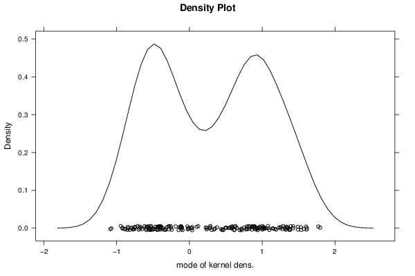
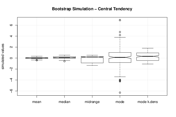
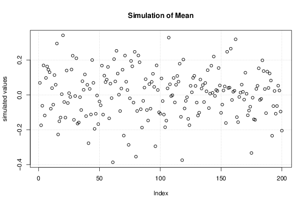
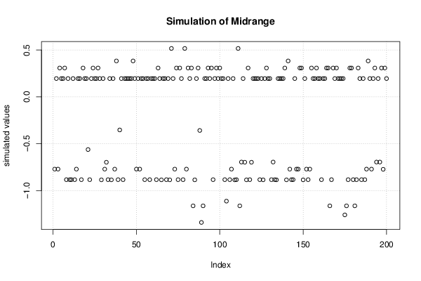
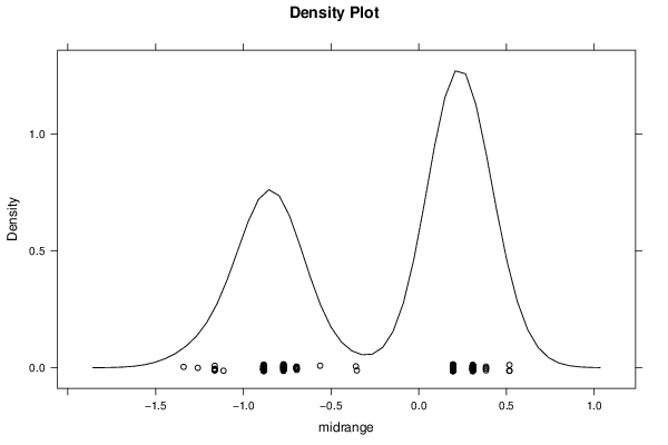
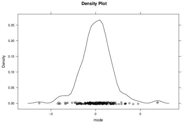
Figures (Output of Computation) | |||||||||||||||||||||||||||||||||||||||||||||||||||||||||||||||||||||||||||||||||||||||||||||||||||||||||||||||||||||||||||||||||||||||||||||||||||||||||||||||||
Input Parameters & R Code | |||||||||||||||||||||||||||||||||||||||||||||||||||||||||||||||||||||||||||||||||||||||||||||||||||||||||||||||||||||||||||||||||||||||||||||||||||||||||||||||||
| Parameters (Session): | |||||||||||||||||||||||||||||||||||||||||||||||||||||||||||||||||||||||||||||||||||||||||||||||||||||||||||||||||||||||||||||||||||||||||||||||||||||||||||||||||
| par1 = 200 ; par2 = 5 ; par3 = 0 ; par4 = P1 P5 Q1 Q3 P95 P99 ; | |||||||||||||||||||||||||||||||||||||||||||||||||||||||||||||||||||||||||||||||||||||||||||||||||||||||||||||||||||||||||||||||||||||||||||||||||||||||||||||||||
| Parameters (R input): | |||||||||||||||||||||||||||||||||||||||||||||||||||||||||||||||||||||||||||||||||||||||||||||||||||||||||||||||||||||||||||||||||||||||||||||||||||||||||||||||||
| par1 = 200 ; par2 = 5 ; par3 = 0 ; par4 = P1 P5 Q1 Q3 P95 P99 ; | |||||||||||||||||||||||||||||||||||||||||||||||||||||||||||||||||||||||||||||||||||||||||||||||||||||||||||||||||||||||||||||||||||||||||||||||||||||||||||||||||
| R code (references can be found in the software module): | |||||||||||||||||||||||||||||||||||||||||||||||||||||||||||||||||||||||||||||||||||||||||||||||||||||||||||||||||||||||||||||||||||||||||||||||||||||||||||||||||
par1 <- as.numeric(par1) | |||||||||||||||||||||||||||||||||||||||||||||||||||||||||||||||||||||||||||||||||||||||||||||||||||||||||||||||||||||||||||||||||||||||||||||||||||||||||||||||||