Free Statistics
of Irreproducible Research!
Description of Statistical Computation | |||||||||||||||||||||||||||||||||||||||||||||||||||||||||||||||||||||||||||||||||||||||||||||||||||||||||||||||||||||||||||||||||||||||||||||||||||||||||||||||||
|---|---|---|---|---|---|---|---|---|---|---|---|---|---|---|---|---|---|---|---|---|---|---|---|---|---|---|---|---|---|---|---|---|---|---|---|---|---|---|---|---|---|---|---|---|---|---|---|---|---|---|---|---|---|---|---|---|---|---|---|---|---|---|---|---|---|---|---|---|---|---|---|---|---|---|---|---|---|---|---|---|---|---|---|---|---|---|---|---|---|---|---|---|---|---|---|---|---|---|---|---|---|---|---|---|---|---|---|---|---|---|---|---|---|---|---|---|---|---|---|---|---|---|---|---|---|---|---|---|---|---|---|---|---|---|---|---|---|---|---|---|---|---|---|---|---|---|---|---|---|---|---|---|---|---|---|---|---|---|---|---|---|
| Author's title | |||||||||||||||||||||||||||||||||||||||||||||||||||||||||||||||||||||||||||||||||||||||||||||||||||||||||||||||||||||||||||||||||||||||||||||||||||||||||||||||||
| Author | *The author of this computation has been verified* | ||||||||||||||||||||||||||||||||||||||||||||||||||||||||||||||||||||||||||||||||||||||||||||||||||||||||||||||||||||||||||||||||||||||||||||||||||||||||||||||||
| R Software Module | rwasp_bootstrapplot1.wasp | ||||||||||||||||||||||||||||||||||||||||||||||||||||||||||||||||||||||||||||||||||||||||||||||||||||||||||||||||||||||||||||||||||||||||||||||||||||||||||||||||
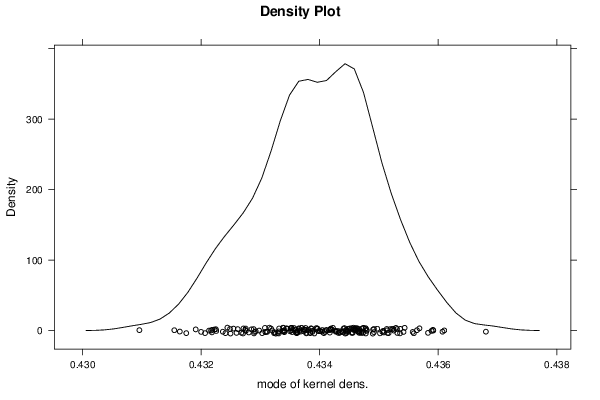
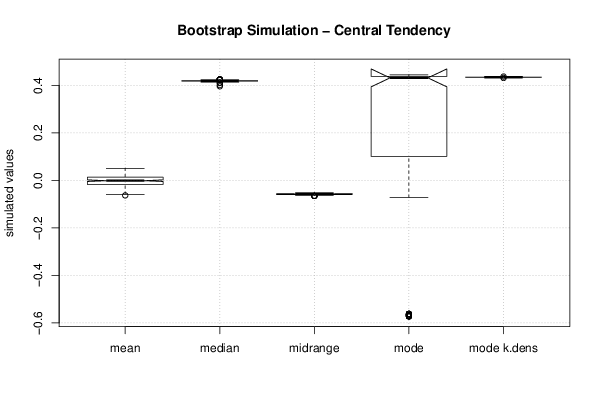
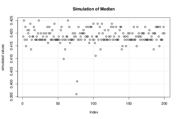
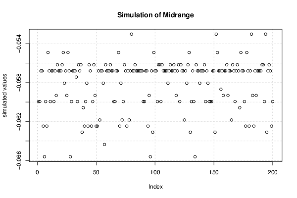
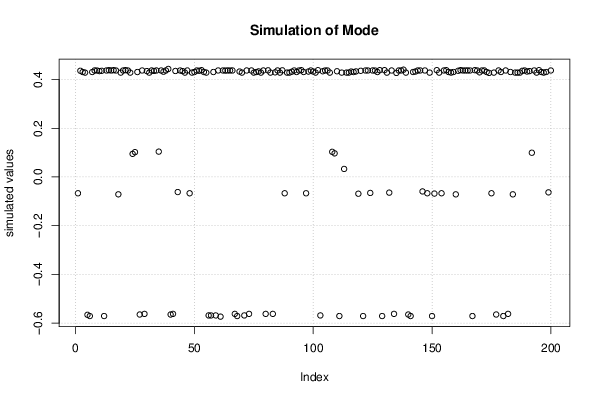
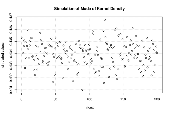
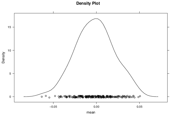
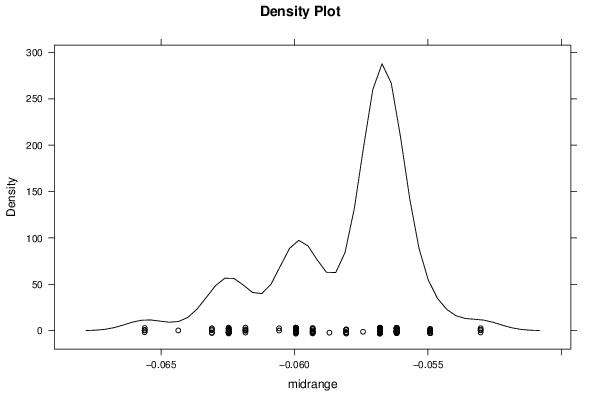
| Title produced by software | Bootstrap Plot - Central Tendency | ||||||||||||||||||||||||||||||||||||||||||||||||||||||||||||||||||||||||||||||||||||||||||||||||||||||||||||||||||||||||||||||||||||||||||||||||||||||||||||||||
| Date of computation | Mon, 15 Dec 2014 10:33:55 +0000 | ||||||||||||||||||||||||||||||||||||||||||||||||||||||||||||||||||||||||||||||||||||||||||||||||||||||||||||||||||||||||||||||||||||||||||||||||||||||||||||||||
| Cite this page as follows | Statistical Computations at FreeStatistics.org, Office for Research Development and Education, URL https://freestatistics.org/blog/index.php?v=date/2014/Dec/15/t14186397182ub2ei70icoykri.htm/, Retrieved Thu, 16 May 2024 13:04:54 +0000 | ||||||||||||||||||||||||||||||||||||||||||||||||||||||||||||||||||||||||||||||||||||||||||||||||||||||||||||||||||||||||||||||||||||||||||||||||||||||||||||||||
| Statistical Computations at FreeStatistics.org, Office for Research Development and Education, URL https://freestatistics.org/blog/index.php?pk=268051, Retrieved Thu, 16 May 2024 13:04:54 +0000 | |||||||||||||||||||||||||||||||||||||||||||||||||||||||||||||||||||||||||||||||||||||||||||||||||||||||||||||||||||||||||||||||||||||||||||||||||||||||||||||||||
| QR Codes: | |||||||||||||||||||||||||||||||||||||||||||||||||||||||||||||||||||||||||||||||||||||||||||||||||||||||||||||||||||||||||||||||||||||||||||||||||||||||||||||||||
|
| |||||||||||||||||||||||||||||||||||||||||||||||||||||||||||||||||||||||||||||||||||||||||||||||||||||||||||||||||||||||||||||||||||||||||||||||||||||||||||||||||
| Original text written by user: | |||||||||||||||||||||||||||||||||||||||||||||||||||||||||||||||||||||||||||||||||||||||||||||||||||||||||||||||||||||||||||||||||||||||||||||||||||||||||||||||||
| IsPrivate? | No (this computation is public) | ||||||||||||||||||||||||||||||||||||||||||||||||||||||||||||||||||||||||||||||||||||||||||||||||||||||||||||||||||||||||||||||||||||||||||||||||||||||||||||||||
| User-defined keywords | |||||||||||||||||||||||||||||||||||||||||||||||||||||||||||||||||||||||||||||||||||||||||||||||||||||||||||||||||||||||||||||||||||||||||||||||||||||||||||||||||
| Estimated Impact | 93 | ||||||||||||||||||||||||||||||||||||||||||||||||||||||||||||||||||||||||||||||||||||||||||||||||||||||||||||||||||||||||||||||||||||||||||||||||||||||||||||||||
Tree of Dependent Computations | |||||||||||||||||||||||||||||||||||||||||||||||||||||||||||||||||||||||||||||||||||||||||||||||||||||||||||||||||||||||||||||||||||||||||||||||||||||||||||||||||
| Family? (F = Feedback message, R = changed R code, M = changed R Module, P = changed Parameters, D = changed Data) | |||||||||||||||||||||||||||||||||||||||||||||||||||||||||||||||||||||||||||||||||||||||||||||||||||||||||||||||||||||||||||||||||||||||||||||||||||||||||||||||||
| - [Bootstrap Plot - Central Tendency] [bootstrap plot] [2014-12-15 10:33:55] [a0dc8dfb1ad11084a66a61bab0a3c2c7] [Current] - RMPD [Mean versus Median] [] [2014-12-18 15:42:11] [be945163e51ed825733188af308451be] - RMPD [Mean versus Median] [] [2014-12-18 15:47:40] [be945163e51ed825733188af308451be] - RMPD [Mean versus Median] [] [2014-12-18 16:00:22] [be945163e51ed825733188af308451be] - RMPD [Bivariate Kernel Density Estimation] [] [2014-12-18 16:46:45] [be945163e51ed825733188af308451be] - RMPD [Histogram] [] [2014-12-18 17:07:51] [be945163e51ed825733188af308451be] - RMPD [Histogram] [] [2014-12-18 17:07:51] [be945163e51ed825733188af308451be] - RMPD [Histogram] [] [2014-12-18 17:27:18] [be945163e51ed825733188af308451be] - RMPD [Histogram] [] [2014-12-18 17:27:41] [be945163e51ed825733188af308451be] - RMPD [Bivariate Kernel Density Estimation] [] [2014-12-18 18:22:19] [be945163e51ed825733188af308451be] - RMPD [Bivariate Kernel Density Estimation] [] [2014-12-18 18:25:23] [be945163e51ed825733188af308451be] | |||||||||||||||||||||||||||||||||||||||||||||||||||||||||||||||||||||||||||||||||||||||||||||||||||||||||||||||||||||||||||||||||||||||||||||||||||||||||||||||||
| Feedback Forum | |||||||||||||||||||||||||||||||||||||||||||||||||||||||||||||||||||||||||||||||||||||||||||||||||||||||||||||||||||||||||||||||||||||||||||||||||||||||||||||||||
Post a new message | |||||||||||||||||||||||||||||||||||||||||||||||||||||||||||||||||||||||||||||||||||||||||||||||||||||||||||||||||||||||||||||||||||||||||||||||||||||||||||||||||
Dataset | |||||||||||||||||||||||||||||||||||||||||||||||||||||||||||||||||||||||||||||||||||||||||||||||||||||||||||||||||||||||||||||||||||||||||||||||||||||||||||||||||
| Dataseries X: | |||||||||||||||||||||||||||||||||||||||||||||||||||||||||||||||||||||||||||||||||||||||||||||||||||||||||||||||||||||||||||||||||||||||||||||||||||||||||||||||||
-0.531003 0.429981 -0.544847 0.417395 0.447601 0.436274 -0.563726 0.447601 0.396 0.417395 0.44005 0.41362 0.436274 -0.571278 -0.583863 -0.576312 0.447601 -0.56876 0.43124 -0.591415 0.419912 0.42243 -0.571278 0.429981 0.42243 0.435015 0.429981 -0.562468 0.421171 -0.564985 -0.534779 -0.566243 0.437532 0.428722 0.447601 0.437532 0.435015 -0.566243 0.43124 0.424947 -0.557433 0.452635 0.441308 0.438791 0.45767 0.463963 -0.583863 0.44005 0.424947 -0.582605 0.442567 0.43124 0.438791 0.447601 0.417395 0.423688 0.429981 -0.549882 0.433757 -0.554916 0.441308 0.424947 -0.56876 -0.549882 0.447601 -0.564985 0.446343 -0.581346 0.428722 0.443825 -0.544847 -0.562468 -0.562468 -0.56876 0.418654 0.445084 -0.544847 0.427464 -0.55114 0.453894 -0.581346 -0.541072 0.435015 -0.55995 -0.567502 -0.55995 0.427464 -0.548623 0.428722 0.426205 -0.57757 -0.56876 -0.566243 0.436274 0.458928 0.414878 -0.538555 0.441308 -0.582605 0.428722 0.429981 0.44886 0.421171 0.428722 -0.581346 0.468997 0.424947 0.436274 -0.562468 -0.567502 -0.561209 -0.573795 -0.56876 -0.57757 0.424947 0.436274 0.481583 0.443825 0.43124 -0.563726 0.432498 0.438791 -0.572536 0.426205 -0.563726 -0.553657 0.417395 0.436274 0.432498 0.455153 0.433757 0.411102 0.437532 0.441308 -0.573795 0.438791 0.42243 0.460187 0.417395 0.443825 0.433757 -0.572536 0.424947 0.460187 0.442567 0.414878 0.436274 -0.567502 -0.567502 -0.549882 0.409844 -0.562468 -0.563726 -0.561209 0.437532 -0.573795 0.43124 0.43124 -0.534779 0.418654 0.418654 0.409844 -0.567502 -0.578829 -0.548623 -0.556175 0.428722 -0.552399 0.424947 -0.562468 0.438791 -0.563726 0.433757 -0.581346 -0.575053 0.401034 -0.562468 0.43124 0.43124 0.43124 0.435015 0.442567 -0.529745 0.442567 -0.556175 -0.561209 -0.547365 0.437532 -0.571278 0.45767 -0.571278 -0.573795 -0.576312 -0.57757 0.435015 0.443825 0.417395 0.427464 -0.578829 -0.546106 0.438791 -0.558692 -0.558692 -0.557433 -0.581346 0.442567 0.42243 -0.571278 -0.553657 0.437532 -0.552399 0.432498 0.453894 0.43124 -0.554916 0.438791 0.433757 0.429981 -0.573795 -0.567502 -0.56876 0.44005 0.455153 -0.552399 0.427464 0.443825 -0.562468 -0.571278 -0.578829 0.435015 0.441308 -0.562468 -0.557433 -0.572536 0.423688 0.423688 -0.562468 -0.578829 -0.563726 0.417395 0.438791 0.433757 0.428722 -0.56876 0.42243 0.462704 0.419912 -0.587639 -0.561209 0.429981 -0.557433 0.433757 0.442567 0.429981 -0.552399 0.450118 -0.57757 0.42243 0.43124 -0.562468 0.438791 -0.525969 0.450118 -0.572536 0.43124 -0.581346 -0.564985 0.44886 0.436274 -0.566243 0.446343 0.423688 -0.564985 0.438791 -0.543589 -0.593932 0.418654 0.423688 -0.572536 0.442567 -0.567502 -0.571278 0.426205 -0.553657 -0.570019 0.445084 0.428722 0.437532 -0.570019 0.463963 0.443825 0.437532 0.43124 -0.571278 0.446343 -0.5159 -0.564985 0.44886 -0.55995 0.446343 -0.576312 -0.536037 0.443825 -0.56876 0.438791 0.433757 -0.558692 -0.567502 -0.54233 0.432498 -0.549882 0.427464 0.433757 0.418654 0.432498 -0.554916 0.437532 -0.557433 0.44886 -0.564985 -0.564985 -0.549882 -0.567502 -0.567502 -0.556175 0.42243 0.447601 0.419912 -0.572536 -0.547365 -0.553657 -0.573795 -0.570019 0.417395 0.436274 0.436274 0.414878 -0.556175 0.443825 -0.564985 0.451377 0.41362 -0.566243 0.40481 -0.554916 -0.573795 -0.557433 -0.561209 -0.581346 -0.573795 0.450118 -0.564985 -0.541072 0.437532 0.414878 0.426205 0.445084 -0.571278 0.452635 0.437532 -0.563726 -0.55995 -0.57757 -0.553657 0.437532 -0.563726 -0.573795 -0.564985 -0.564985 -0.563726 -0.537296 0.437532 0.419912 0.437532 -0.55995 -0.575053 0.428722 -0.576312 0.433757 0.436274 0.411102 0.438791 0.419912 -0.564985 -0.56876 -0.57757 -0.576312 -0.581346 0.438791 -0.554916 -0.571278 0.436274 -0.564985 -0.583863 0.427464 -0.571278 0.436274 0.445084 -0.571278 0.41362 -0.585122 0.412361 -0.556175 0.428722 0.452635 0.443825 -0.578829 0.417395 0.446343 -0.566243 0.450118 0.416137 0.42243 0.429981 -0.575053 0.452635 -0.585122 -0.578829 0.453894 -0.572536 0.437532 0.427464 -0.562468 -0.580088 0.442567 0.438791 0.429981 0.47529 -0.557433 0.437532 0.455153 0.417395 0.447601 -0.571278 -0.562468 0.451377 -0.549882 0.428722 0.421171 -0.578829 0.428722 -0.561209 0.427464 -0.567502 -0.572536 0.428722 0.450118 0.43124 0.42243 -0.59519 -0.573795 0.428722 -0.578829 0.442567 -0.556175 0.423688 0.426205 0.438791 0.443825 0.446343 0.428722 0.43124 0.447601 -0.566243 0.433757 -0.56876 -0.580088 0.418654 0.423688 0.428722 0.417395 0.470255 0.43124 0.435015 -0.56876 0.427464 0.443825 0.44005 -0.56876 0.406068 0.460187 0.44005 0.435015 -0.571278 0.411102 0.437532 -0.55114 -0.585122 0.437532 0.433757 0.436274 0.427464 -0.562468 0.417395 -0.578829 0.428722 0.435015 | |||||||||||||||||||||||||||||||||||||||||||||||||||||||||||||||||||||||||||||||||||||||||||||||||||||||||||||||||||||||||||||||||||||||||||||||||||||||||||||||||
Tables (Output of Computation) | |||||||||||||||||||||||||||||||||||||||||||||||||||||||||||||||||||||||||||||||||||||||||||||||||||||||||||||||||||||||||||||||||||||||||||||||||||||||||||||||||
| |||||||||||||||||||||||||||||||||||||||||||||||||||||||||||||||||||||||||||||||||||||||||||||||||||||||||||||||||||||||||||||||||||||||||||||||||||||||||||||||||
Figures (Output of Computation) | |||||||||||||||||||||||||||||||||||||||||||||||||||||||||||||||||||||||||||||||||||||||||||||||||||||||||||||||||||||||||||||||||||||||||||||||||||||||||||||||||
Input Parameters & R Code | |||||||||||||||||||||||||||||||||||||||||||||||||||||||||||||||||||||||||||||||||||||||||||||||||||||||||||||||||||||||||||||||||||||||||||||||||||||||||||||||||
| Parameters (Session): | |||||||||||||||||||||||||||||||||||||||||||||||||||||||||||||||||||||||||||||||||||||||||||||||||||||||||||||||||||||||||||||||||||||||||||||||||||||||||||||||||
| par1 = 200 ; par2 = 5 ; par3 = 0 ; par4 = P1 P5 Q1 Q3 P95 P99 ; | |||||||||||||||||||||||||||||||||||||||||||||||||||||||||||||||||||||||||||||||||||||||||||||||||||||||||||||||||||||||||||||||||||||||||||||||||||||||||||||||||
| Parameters (R input): | |||||||||||||||||||||||||||||||||||||||||||||||||||||||||||||||||||||||||||||||||||||||||||||||||||||||||||||||||||||||||||||||||||||||||||||||||||||||||||||||||
| par1 = 200 ; par2 = 5 ; par3 = 0 ; par4 = P1 P5 Q1 Q3 P95 P99 ; | |||||||||||||||||||||||||||||||||||||||||||||||||||||||||||||||||||||||||||||||||||||||||||||||||||||||||||||||||||||||||||||||||||||||||||||||||||||||||||||||||
| R code (references can be found in the software module): | |||||||||||||||||||||||||||||||||||||||||||||||||||||||||||||||||||||||||||||||||||||||||||||||||||||||||||||||||||||||||||||||||||||||||||||||||||||||||||||||||
par1 <- as.numeric(par1) | |||||||||||||||||||||||||||||||||||||||||||||||||||||||||||||||||||||||||||||||||||||||||||||||||||||||||||||||||||||||||||||||||||||||||||||||||||||||||||||||||