Free Statistics
of Irreproducible Research!
Description of Statistical Computation | |||||||||||||||||||||||||||||||||||||||||||||||||||||||||||||||||||||||||||||||||||||||||||||||||||||||||||||||||||||||||||||||||||||||||||||||||||||||||||||||||||||||||||||||||
|---|---|---|---|---|---|---|---|---|---|---|---|---|---|---|---|---|---|---|---|---|---|---|---|---|---|---|---|---|---|---|---|---|---|---|---|---|---|---|---|---|---|---|---|---|---|---|---|---|---|---|---|---|---|---|---|---|---|---|---|---|---|---|---|---|---|---|---|---|---|---|---|---|---|---|---|---|---|---|---|---|---|---|---|---|---|---|---|---|---|---|---|---|---|---|---|---|---|---|---|---|---|---|---|---|---|---|---|---|---|---|---|---|---|---|---|---|---|---|---|---|---|---|---|---|---|---|---|---|---|---|---|---|---|---|---|---|---|---|---|---|---|---|---|---|---|---|---|---|---|---|---|---|---|---|---|---|---|---|---|---|---|---|---|---|---|---|---|---|---|---|---|---|---|---|---|---|---|
| Author's title | |||||||||||||||||||||||||||||||||||||||||||||||||||||||||||||||||||||||||||||||||||||||||||||||||||||||||||||||||||||||||||||||||||||||||||||||||||||||||||||||||||||||||||||||||
| Author | *The author of this computation has been verified* | ||||||||||||||||||||||||||||||||||||||||||||||||||||||||||||||||||||||||||||||||||||||||||||||||||||||||||||||||||||||||||||||||||||||||||||||||||||||||||||||||||||||||||||||||
| R Software Module | rwasp_twosampletests_mean.wasp | ||||||||||||||||||||||||||||||||||||||||||||||||||||||||||||||||||||||||||||||||||||||||||||||||||||||||||||||||||||||||||||||||||||||||||||||||||||||||||||||||||||||||||||||||
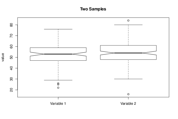
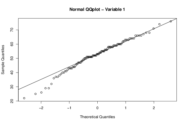
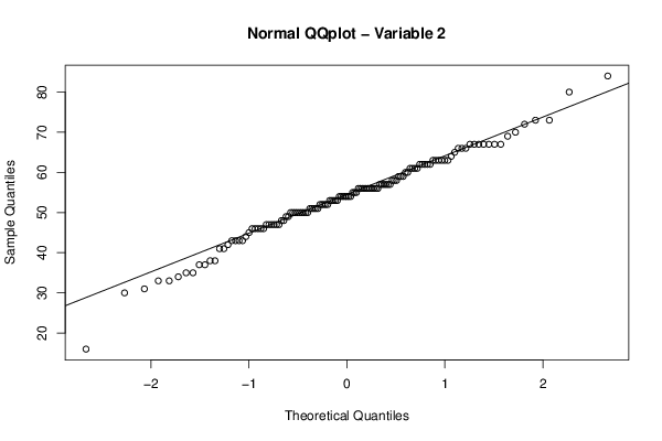
| Title produced by software | Paired and Unpaired Two Samples Tests about the Mean | ||||||||||||||||||||||||||||||||||||||||||||||||||||||||||||||||||||||||||||||||||||||||||||||||||||||||||||||||||||||||||||||||||||||||||||||||||||||||||||||||||||||||||||||||
| Date of computation | Mon, 15 Dec 2014 16:32:47 +0000 | ||||||||||||||||||||||||||||||||||||||||||||||||||||||||||||||||||||||||||||||||||||||||||||||||||||||||||||||||||||||||||||||||||||||||||||||||||||||||||||||||||||||||||||||||
| Cite this page as follows | Statistical Computations at FreeStatistics.org, Office for Research Development and Education, URL https://freestatistics.org/blog/index.php?v=date/2014/Dec/15/t1418661182o7m65r71z6o0hyw.htm/, Retrieved Thu, 16 May 2024 09:29:36 +0000 | ||||||||||||||||||||||||||||||||||||||||||||||||||||||||||||||||||||||||||||||||||||||||||||||||||||||||||||||||||||||||||||||||||||||||||||||||||||||||||||||||||||||||||||||||
| Statistical Computations at FreeStatistics.org, Office for Research Development and Education, URL https://freestatistics.org/blog/index.php?pk=268723, Retrieved Thu, 16 May 2024 09:29:36 +0000 | |||||||||||||||||||||||||||||||||||||||||||||||||||||||||||||||||||||||||||||||||||||||||||||||||||||||||||||||||||||||||||||||||||||||||||||||||||||||||||||||||||||||||||||||||
| QR Codes: | |||||||||||||||||||||||||||||||||||||||||||||||||||||||||||||||||||||||||||||||||||||||||||||||||||||||||||||||||||||||||||||||||||||||||||||||||||||||||||||||||||||||||||||||||
|
| |||||||||||||||||||||||||||||||||||||||||||||||||||||||||||||||||||||||||||||||||||||||||||||||||||||||||||||||||||||||||||||||||||||||||||||||||||||||||||||||||||||||||||||||||
| Original text written by user: | |||||||||||||||||||||||||||||||||||||||||||||||||||||||||||||||||||||||||||||||||||||||||||||||||||||||||||||||||||||||||||||||||||||||||||||||||||||||||||||||||||||||||||||||||
| IsPrivate? | No (this computation is public) | ||||||||||||||||||||||||||||||||||||||||||||||||||||||||||||||||||||||||||||||||||||||||||||||||||||||||||||||||||||||||||||||||||||||||||||||||||||||||||||||||||||||||||||||||
| User-defined keywords | |||||||||||||||||||||||||||||||||||||||||||||||||||||||||||||||||||||||||||||||||||||||||||||||||||||||||||||||||||||||||||||||||||||||||||||||||||||||||||||||||||||||||||||||||
| Estimated Impact | 87 | ||||||||||||||||||||||||||||||||||||||||||||||||||||||||||||||||||||||||||||||||||||||||||||||||||||||||||||||||||||||||||||||||||||||||||||||||||||||||||||||||||||||||||||||||
Tree of Dependent Computations | |||||||||||||||||||||||||||||||||||||||||||||||||||||||||||||||||||||||||||||||||||||||||||||||||||||||||||||||||||||||||||||||||||||||||||||||||||||||||||||||||||||||||||||||||
| Family? (F = Feedback message, R = changed R code, M = changed R Module, P = changed Parameters, D = changed Data) | |||||||||||||||||||||||||||||||||||||||||||||||||||||||||||||||||||||||||||||||||||||||||||||||||||||||||||||||||||||||||||||||||||||||||||||||||||||||||||||||||||||||||||||||||
| - [Paired and Unpaired Two Samples Tests about the Mean] [] [2014-12-15 16:20:32] [67894a4ff6098ffac356bc81e6028257] - D [Paired and Unpaired Two Samples Tests about the Mean] [] [2014-12-15 16:32:47] [9a966322e4d935aee68609d815c1a240] [Current] - RMPD [One-Way-Between-Groups ANOVA- Free Statistics Software (Calculator)] [] [2014-12-18 16:14:55] [67894a4ff6098ffac356bc81e6028257] - RMPD [One-Way-Between-Groups ANOVA- Free Statistics Software (Calculator)] [] [2014-12-18 16:17:59] [67894a4ff6098ffac356bc81e6028257] - RMPD [Two-Way ANOVA] [] [2014-12-18 16:25:08] [67894a4ff6098ffac356bc81e6028257] - RMPD [Multiple Regression] [] [2014-12-18 17:11:06] [67894a4ff6098ffac356bc81e6028257] - RMPD [Chi-Squared Test, McNemar Test, and Fisher Exact Test] [] [2014-12-18 17:33:22] [67894a4ff6098ffac356bc81e6028257] - RM D [Chi-Squared Test, McNemar Test, and Fisher Exact Test] [] [2014-12-18 17:37:05] [67894a4ff6098ffac356bc81e6028257] - RM D [Chi-Squared Test, McNemar Test, and Fisher Exact Test] [] [2014-12-18 17:45:31] [67894a4ff6098ffac356bc81e6028257] | |||||||||||||||||||||||||||||||||||||||||||||||||||||||||||||||||||||||||||||||||||||||||||||||||||||||||||||||||||||||||||||||||||||||||||||||||||||||||||||||||||||||||||||||||
| Feedback Forum | |||||||||||||||||||||||||||||||||||||||||||||||||||||||||||||||||||||||||||||||||||||||||||||||||||||||||||||||||||||||||||||||||||||||||||||||||||||||||||||||||||||||||||||||||
Post a new message | |||||||||||||||||||||||||||||||||||||||||||||||||||||||||||||||||||||||||||||||||||||||||||||||||||||||||||||||||||||||||||||||||||||||||||||||||||||||||||||||||||||||||||||||||
Dataset | |||||||||||||||||||||||||||||||||||||||||||||||||||||||||||||||||||||||||||||||||||||||||||||||||||||||||||||||||||||||||||||||||||||||||||||||||||||||||||||||||||||||||||||||||
| Dataseries X: | |||||||||||||||||||||||||||||||||||||||||||||||||||||||||||||||||||||||||||||||||||||||||||||||||||||||||||||||||||||||||||||||||||||||||||||||||||||||||||||||||||||||||||||||||
26 NA 51 NA NA 57 37 NA NA 67 NA 43 NA 52 52 NA NA 43 NA 84 NA 67 NA 49 NA 70 58 NA 68 NA 62 NA NA 43 56 NA 74 NA NA 63 58 NA NA 63 NA 53 NA 57 NA 64 53 NA 29 NA 54 NA NA 58 NA 51 54 NA NA 56 47 NA NA 50 NA 35 NA 30 68 NA NA 56 NA 43 NA 67 NA 62 NA 57 NA 54 NA 61 56 NA 41 NA 53 NA NA 46 51 NA 37 NA 42 NA NA 38 66 NA NA 53 49 NA 49 NA NA 59 40 NA 63 NA NA 34 32 NA 67 NA NA 61 60 NA 63 NA NA 52 NA 16 NA 46 NA 56 52 NA NA 55 NA 50 59 NA NA 60 52 NA 44 NA NA 67 NA 52 NA 55 NA 37 NA 54 NA 72 NA 51 NA 48 60 NA NA 50 NA 63 NA 33 NA 67 NA 46 NA 54 59 NA NA 61 NA 33 NA 47 NA 69 NA 52 55 NA 55 NA 41 NA NA 73 51 NA 52 NA 50 NA NA 51 60 NA NA 56 NA 56 29 NA NA 66 NA 66 NA 73 55 NA 64 NA 40 NA 46 NA NA 58 43 NA NA 61 51 NA NA 50 52 NA NA 54 66 NA 61 NA NA 80 51 NA NA 56 NA 56 NA 56 NA 53 NA 47 25 NA NA 47 46 NA 50 NA 39 NA NA 51 58 NA NA 35 58 NA 60 NA 62 NA 63 NA NA 53 NA 46 NA 67 NA 59 64 NA 38 NA NA 50 48 NA 48 NA 47 NA 66 NA NA 47 NA 63 58 NA 44 NA NA 51 43 NA NA 55 NA 38 NA 56 45 NA NA 50 NA 54 NA 57 60 NA 55 NA 56 NA NA 49 NA 37 43 NA NA 59 NA 46 51 NA 58 NA 64 NA NA 53 NA 48 51 NA 47 NA 59 NA NA 62 NA 62 51 NA 64 NA 52 NA NA 67 NA 50 NA 54 NA 58 56 NA NA 63 NA 31 NA 65 71 NA 50 NA NA 57 47 NA NA 54 NA 47 NA 57 43 NA NA 41 63 NA NA 63 NA 56 51 NA NA 50 22 NA NA 41 59 NA NA 56 66 NA 53 NA NA 42 NA 52 54 NA NA 44 NA 62 53 NA NA 50 36 NA 76 NA NA 66 NA 62 59 NA NA 47 55 NA 58 NA NA 60 44 NA 57 NA NA 45 | |||||||||||||||||||||||||||||||||||||||||||||||||||||||||||||||||||||||||||||||||||||||||||||||||||||||||||||||||||||||||||||||||||||||||||||||||||||||||||||||||||||||||||||||||
Tables (Output of Computation) | |||||||||||||||||||||||||||||||||||||||||||||||||||||||||||||||||||||||||||||||||||||||||||||||||||||||||||||||||||||||||||||||||||||||||||||||||||||||||||||||||||||||||||||||||
| |||||||||||||||||||||||||||||||||||||||||||||||||||||||||||||||||||||||||||||||||||||||||||||||||||||||||||||||||||||||||||||||||||||||||||||||||||||||||||||||||||||||||||||||||
Figures (Output of Computation) | |||||||||||||||||||||||||||||||||||||||||||||||||||||||||||||||||||||||||||||||||||||||||||||||||||||||||||||||||||||||||||||||||||||||||||||||||||||||||||||||||||||||||||||||||
Input Parameters & R Code | |||||||||||||||||||||||||||||||||||||||||||||||||||||||||||||||||||||||||||||||||||||||||||||||||||||||||||||||||||||||||||||||||||||||||||||||||||||||||||||||||||||||||||||||||
| Parameters (Session): | |||||||||||||||||||||||||||||||||||||||||||||||||||||||||||||||||||||||||||||||||||||||||||||||||||||||||||||||||||||||||||||||||||||||||||||||||||||||||||||||||||||||||||||||||
| Parameters (R input): | |||||||||||||||||||||||||||||||||||||||||||||||||||||||||||||||||||||||||||||||||||||||||||||||||||||||||||||||||||||||||||||||||||||||||||||||||||||||||||||||||||||||||||||||||
| par1 = 1 ; par2 = 2 ; par3 = 0.95 ; par4 = two.sided ; par5 = unpaired ; par6 = 0 ; | |||||||||||||||||||||||||||||||||||||||||||||||||||||||||||||||||||||||||||||||||||||||||||||||||||||||||||||||||||||||||||||||||||||||||||||||||||||||||||||||||||||||||||||||||
| R code (references can be found in the software module): | |||||||||||||||||||||||||||||||||||||||||||||||||||||||||||||||||||||||||||||||||||||||||||||||||||||||||||||||||||||||||||||||||||||||||||||||||||||||||||||||||||||||||||||||||
par1 <- as.numeric(par1) #column number of first sample | |||||||||||||||||||||||||||||||||||||||||||||||||||||||||||||||||||||||||||||||||||||||||||||||||||||||||||||||||||||||||||||||||||||||||||||||||||||||||||||||||||||||||||||||||