Free Statistics
of Irreproducible Research!
Description of Statistical Computation | |||||||||||||||||||||||||||||||||||||||||||||||||||||||||||||||||||||||||||||||||||||||||||||||||||||||||||||||||||||||||||||||||||||||||||||||||||||||||||||||||
|---|---|---|---|---|---|---|---|---|---|---|---|---|---|---|---|---|---|---|---|---|---|---|---|---|---|---|---|---|---|---|---|---|---|---|---|---|---|---|---|---|---|---|---|---|---|---|---|---|---|---|---|---|---|---|---|---|---|---|---|---|---|---|---|---|---|---|---|---|---|---|---|---|---|---|---|---|---|---|---|---|---|---|---|---|---|---|---|---|---|---|---|---|---|---|---|---|---|---|---|---|---|---|---|---|---|---|---|---|---|---|---|---|---|---|---|---|---|---|---|---|---|---|---|---|---|---|---|---|---|---|---|---|---|---|---|---|---|---|---|---|---|---|---|---|---|---|---|---|---|---|---|---|---|---|---|---|---|---|---|---|---|
| Author's title | |||||||||||||||||||||||||||||||||||||||||||||||||||||||||||||||||||||||||||||||||||||||||||||||||||||||||||||||||||||||||||||||||||||||||||||||||||||||||||||||||
| Author | *The author of this computation has been verified* | ||||||||||||||||||||||||||||||||||||||||||||||||||||||||||||||||||||||||||||||||||||||||||||||||||||||||||||||||||||||||||||||||||||||||||||||||||||||||||||||||
| R Software Module | rwasp_bootstrapplot1.wasp | ||||||||||||||||||||||||||||||||||||||||||||||||||||||||||||||||||||||||||||||||||||||||||||||||||||||||||||||||||||||||||||||||||||||||||||||||||||||||||||||||
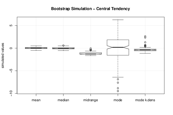
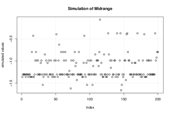
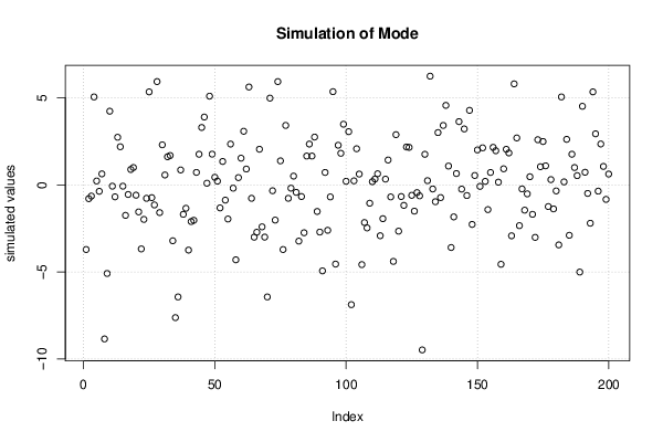
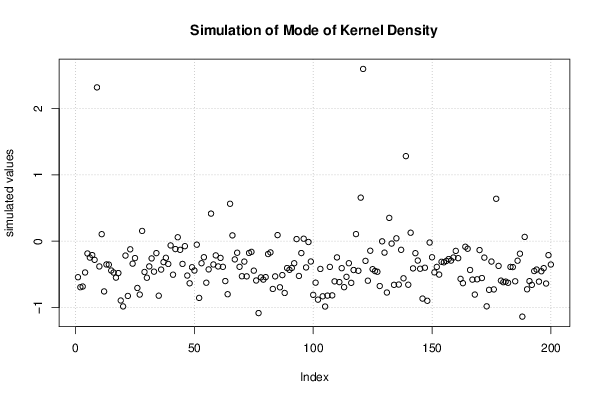
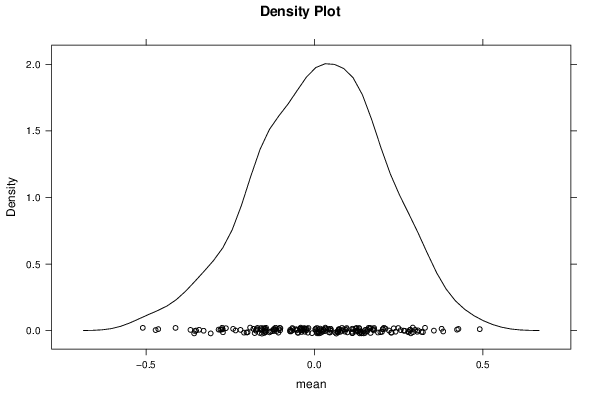
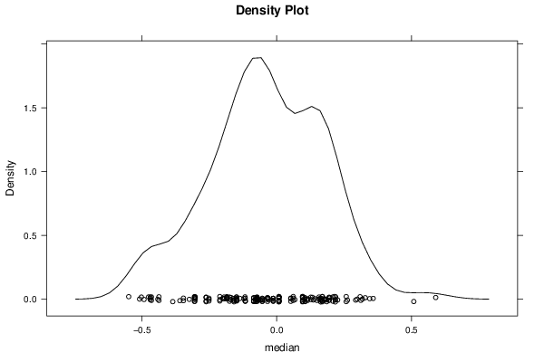
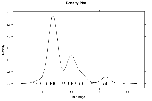
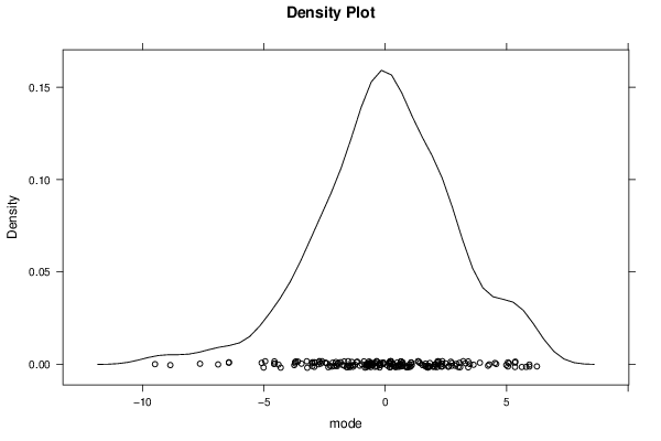
| Title produced by software | Bootstrap Plot - Central Tendency | ||||||||||||||||||||||||||||||||||||||||||||||||||||||||||||||||||||||||||||||||||||||||||||||||||||||||||||||||||||||||||||||||||||||||||||||||||||||||||||||||
| Date of computation | Mon, 15 Dec 2014 17:13:54 +0000 | ||||||||||||||||||||||||||||||||||||||||||||||||||||||||||||||||||||||||||||||||||||||||||||||||||||||||||||||||||||||||||||||||||||||||||||||||||||||||||||||||
| Cite this page as follows | Statistical Computations at FreeStatistics.org, Office for Research Development and Education, URL https://freestatistics.org/blog/index.php?v=date/2014/Dec/15/t14186637497igsbnrj2gaquqq.htm/, Retrieved Thu, 16 May 2024 22:34:47 +0000 | ||||||||||||||||||||||||||||||||||||||||||||||||||||||||||||||||||||||||||||||||||||||||||||||||||||||||||||||||||||||||||||||||||||||||||||||||||||||||||||||||
| Statistical Computations at FreeStatistics.org, Office for Research Development and Education, URL https://freestatistics.org/blog/index.php?pk=268771, Retrieved Thu, 16 May 2024 22:34:47 +0000 | |||||||||||||||||||||||||||||||||||||||||||||||||||||||||||||||||||||||||||||||||||||||||||||||||||||||||||||||||||||||||||||||||||||||||||||||||||||||||||||||||
| QR Codes: | |||||||||||||||||||||||||||||||||||||||||||||||||||||||||||||||||||||||||||||||||||||||||||||||||||||||||||||||||||||||||||||||||||||||||||||||||||||||||||||||||
|
| |||||||||||||||||||||||||||||||||||||||||||||||||||||||||||||||||||||||||||||||||||||||||||||||||||||||||||||||||||||||||||||||||||||||||||||||||||||||||||||||||
| Original text written by user: | |||||||||||||||||||||||||||||||||||||||||||||||||||||||||||||||||||||||||||||||||||||||||||||||||||||||||||||||||||||||||||||||||||||||||||||||||||||||||||||||||
| IsPrivate? | No (this computation is public) | ||||||||||||||||||||||||||||||||||||||||||||||||||||||||||||||||||||||||||||||||||||||||||||||||||||||||||||||||||||||||||||||||||||||||||||||||||||||||||||||||
| User-defined keywords | |||||||||||||||||||||||||||||||||||||||||||||||||||||||||||||||||||||||||||||||||||||||||||||||||||||||||||||||||||||||||||||||||||||||||||||||||||||||||||||||||
| Estimated Impact | 71 | ||||||||||||||||||||||||||||||||||||||||||||||||||||||||||||||||||||||||||||||||||||||||||||||||||||||||||||||||||||||||||||||||||||||||||||||||||||||||||||||||
Tree of Dependent Computations | |||||||||||||||||||||||||||||||||||||||||||||||||||||||||||||||||||||||||||||||||||||||||||||||||||||||||||||||||||||||||||||||||||||||||||||||||||||||||||||||||
| Family? (F = Feedback message, R = changed R code, M = changed R Module, P = changed Parameters, D = changed Data) | |||||||||||||||||||||||||||||||||||||||||||||||||||||||||||||||||||||||||||||||||||||||||||||||||||||||||||||||||||||||||||||||||||||||||||||||||||||||||||||||||
| - [Central Tendency] [] [2014-11-04 10:08:09] [32b17a345b130fdf5cc88718ed94a974] - [Central Tendency] [WS7 3] [2014-11-12 20:26:33] [81f624c2f0b20a2549c93e7c3dccf981] - D [Central Tendency] [] [2014-12-15 16:40:00] [ae96d02647dd9ad9c105f1fa6642e295] - RM D [Bootstrap Plot - Central Tendency] [] [2014-12-15 17:13:54] [4ade5e15fc88dfcb6333f94ac70b9a75] [Current] | |||||||||||||||||||||||||||||||||||||||||||||||||||||||||||||||||||||||||||||||||||||||||||||||||||||||||||||||||||||||||||||||||||||||||||||||||||||||||||||||||
| Feedback Forum | |||||||||||||||||||||||||||||||||||||||||||||||||||||||||||||||||||||||||||||||||||||||||||||||||||||||||||||||||||||||||||||||||||||||||||||||||||||||||||||||||
Post a new message | |||||||||||||||||||||||||||||||||||||||||||||||||||||||||||||||||||||||||||||||||||||||||||||||||||||||||||||||||||||||||||||||||||||||||||||||||||||||||||||||||
Dataset | |||||||||||||||||||||||||||||||||||||||||||||||||||||||||||||||||||||||||||||||||||||||||||||||||||||||||||||||||||||||||||||||||||||||||||||||||||||||||||||||||
| Dataseries X: | |||||||||||||||||||||||||||||||||||||||||||||||||||||||||||||||||||||||||||||||||||||||||||||||||||||||||||||||||||||||||||||||||||||||||||||||||||||||||||||||||
-0.531142 -1.13262 -0.582415 -5.59232 -6.83235 -0.305178 2.34674 -0.147607 -1.45216 -6.53672 -1.47258 -7.01355 -1.5525 -0.691061 -6.47182 -1.3266 -0.910526 -3.5313 -3.71408 -2.47297 -6.55211 0.884966 -1.98207 1.06889 -1.24589 -1.87098 3.21616 0.303614 -3.27261 -0.910074 -3.90055 -1.45827 -3.66334 -2.90078 -1.75345 -2.92291 -2.39109 -0.345755 -4.26578 -0.489436 -7.67222 -1.93212 0.169032 -1.24816 -0.221419 -1.95304 -1.46435 -5.09199 0.00843549 -0.771406 -0.930545 -6.31456 -2.27144 -0.772019 -0.0730031 -2.75141 -6.44107 1.50264 -5.03119 0.208487 -3.99275 -0.302012 -4.30674 2.81801 -3.99675 -3.82478 -1.63475 -0.412881 1.65845 -0.61019 -0.945981 -1.69168 -4.45707 0.72551 0.631932 0.357607 -0.501763 -0.0729741 -2.60926 -5.01083 -2.43116 0.769258 -1.67025 -8.47289 -2.69552 -1.34455 -1.95234 -1.09084 -4.26373 0.589365 -0.514924 -6.88468 -3.25441 -3.55659 -5.54268 -3.99232 -5.75511 -1.42526 0.689277 -4.85155 -2.20238 -2.37146 -4.01912 -3.21153 1.26867 -4.56396 0.202885 -7.63021 -6.72304 -3.71252 -1.4322 -2.07244 -9.48517 -0.169168 5.40647 4.98784 3.06715 -0.672529 3.48706 5.78732 3.12498 0.298365 4.51436 2.00844 -2.51179 -0.302208 3.47768 0.508152 5.80715 1.03604 1.43307 3.20584 2.15964 1.82795 -0.460219 -0.943839 4.23855 -4.13094 5.62711 2.14245 -1.05444 5.09965 2.45493 5.31862 3.4185 3.88483 -0.655842 0.997607 1.37767 4.91301 -2.41178 2.59647 4.84647 3.8999 1.08642 0.185256 5.26481 2.87825 1.10517 -1.00021 5.45728 2.96833 3.80826 2.5065 5.99235 -1.59119 5.93816 2.15775 1.42627 -1.4971 2.9369 5.06377 1.76713 1.96404 2.08435 5.12821 -0.0854529 6.41078 2.27859 -4.94393 0.113974 0.717979 6.24893 2.49879 0.331927 2.92302 4.28397 0.225781 -0.916197 0.0079025 -2.76145 2.73616 -4.01344 5.05511 0.228339 1.07806 2.19985 1.09479 1.88875 2.85672 4.23492 -0.57508 0.608181 3.05997 0.589885 1.96993 -2.90105 -0.90839 6.77032 4.18853 -1.77311 2.48803 -0.771123 0.870016 3.81945 -1.13739 2.88708 5.25838 -1.45252 2.61847 5.3597 -4.62661 -1.05336 3.16702 6.62781 2.50938 3.78732 2.7375 5.68866 6.16807 5.34653 5.92649 0.649042 0.31979 -3.47155 -8.8543 -0.683682 1.04431 -2.9144 -0.643121 0.156948 -0.468542 1.68768 6.87933 -2.02414 2.2298 4.24811 1.21169 3.03694 0.28694 -0.771557 -0.811631 1.94676 2.84017 0.721034 3.71777 -4.7407 -4.58283 0.0957772 -5.5728 -2.77115 -0.200484 -3.3111 1.7629 3.60755 -0.0340522 0.377945 3.06808 3.63718 -1.97265 2.69898 -0.149587 2.31809 4.81833 1.98751 1.13699 3.97591 -4.48868 | |||||||||||||||||||||||||||||||||||||||||||||||||||||||||||||||||||||||||||||||||||||||||||||||||||||||||||||||||||||||||||||||||||||||||||||||||||||||||||||||||
Tables (Output of Computation) | |||||||||||||||||||||||||||||||||||||||||||||||||||||||||||||||||||||||||||||||||||||||||||||||||||||||||||||||||||||||||||||||||||||||||||||||||||||||||||||||||
| |||||||||||||||||||||||||||||||||||||||||||||||||||||||||||||||||||||||||||||||||||||||||||||||||||||||||||||||||||||||||||||||||||||||||||||||||||||||||||||||||
Figures (Output of Computation) | |||||||||||||||||||||||||||||||||||||||||||||||||||||||||||||||||||||||||||||||||||||||||||||||||||||||||||||||||||||||||||||||||||||||||||||||||||||||||||||||||
Input Parameters & R Code | |||||||||||||||||||||||||||||||||||||||||||||||||||||||||||||||||||||||||||||||||||||||||||||||||||||||||||||||||||||||||||||||||||||||||||||||||||||||||||||||||
| Parameters (Session): | |||||||||||||||||||||||||||||||||||||||||||||||||||||||||||||||||||||||||||||||||||||||||||||||||||||||||||||||||||||||||||||||||||||||||||||||||||||||||||||||||
| Parameters (R input): | |||||||||||||||||||||||||||||||||||||||||||||||||||||||||||||||||||||||||||||||||||||||||||||||||||||||||||||||||||||||||||||||||||||||||||||||||||||||||||||||||
| par1 = 200 ; par2 = 5 ; par3 = 0 ; par4 = P1 P5 Q1 Q3 P95 P99 ; | |||||||||||||||||||||||||||||||||||||||||||||||||||||||||||||||||||||||||||||||||||||||||||||||||||||||||||||||||||||||||||||||||||||||||||||||||||||||||||||||||
| R code (references can be found in the software module): | |||||||||||||||||||||||||||||||||||||||||||||||||||||||||||||||||||||||||||||||||||||||||||||||||||||||||||||||||||||||||||||||||||||||||||||||||||||||||||||||||
par1 <- as.numeric(par1) | |||||||||||||||||||||||||||||||||||||||||||||||||||||||||||||||||||||||||||||||||||||||||||||||||||||||||||||||||||||||||||||||||||||||||||||||||||||||||||||||||