Free Statistics
of Irreproducible Research!
Description of Statistical Computation | |||||||||||||||||||||||||||||||||||||||||||||||||||||||||||||||||||||||||||||||||||||||
|---|---|---|---|---|---|---|---|---|---|---|---|---|---|---|---|---|---|---|---|---|---|---|---|---|---|---|---|---|---|---|---|---|---|---|---|---|---|---|---|---|---|---|---|---|---|---|---|---|---|---|---|---|---|---|---|---|---|---|---|---|---|---|---|---|---|---|---|---|---|---|---|---|---|---|---|---|---|---|---|---|---|---|---|---|---|---|---|
| Author's title | |||||||||||||||||||||||||||||||||||||||||||||||||||||||||||||||||||||||||||||||||||||||
| Author | *The author of this computation has been verified* | ||||||||||||||||||||||||||||||||||||||||||||||||||||||||||||||||||||||||||||||||||||||
| R Software Module | rwasp_density.wasp | ||||||||||||||||||||||||||||||||||||||||||||||||||||||||||||||||||||||||||||||||||||||
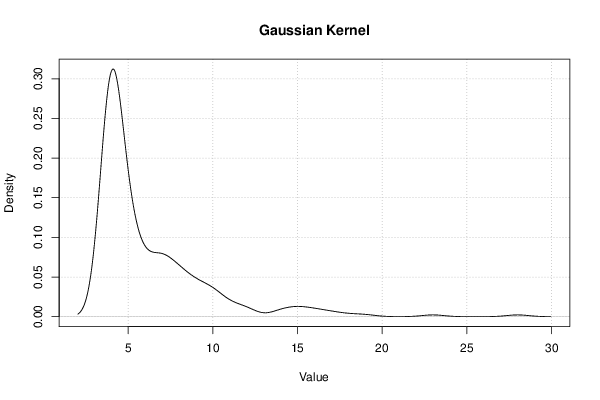
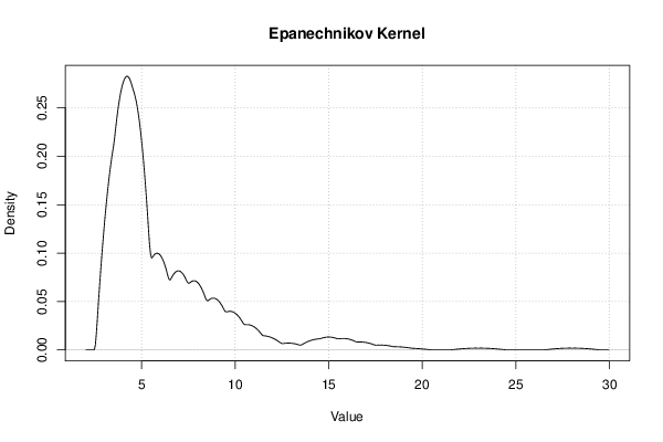
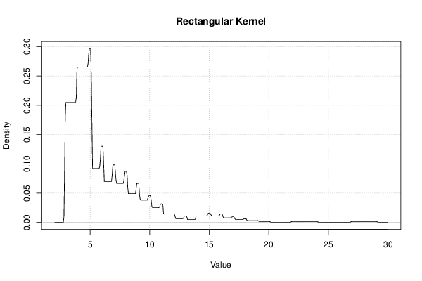
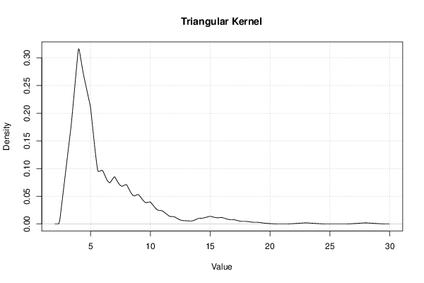
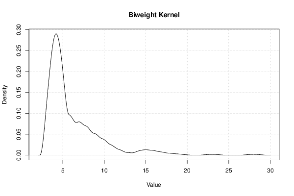
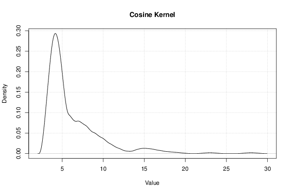
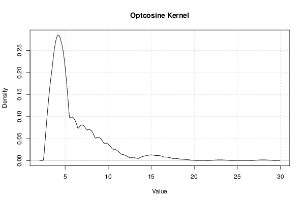
| Title produced by software | Kernel Density Estimation | ||||||||||||||||||||||||||||||||||||||||||||||||||||||||||||||||||||||||||||||||||||||
| Date of computation | Mon, 15 Dec 2014 18:53:06 +0000 | ||||||||||||||||||||||||||||||||||||||||||||||||||||||||||||||||||||||||||||||||||||||
| Cite this page as follows | Statistical Computations at FreeStatistics.org, Office for Research Development and Education, URL https://freestatistics.org/blog/index.php?v=date/2014/Dec/15/t1418669593t05p3kxjhnmi1hi.htm/, Retrieved Thu, 16 May 2024 06:54:16 +0000 | ||||||||||||||||||||||||||||||||||||||||||||||||||||||||||||||||||||||||||||||||||||||
| Statistical Computations at FreeStatistics.org, Office for Research Development and Education, URL https://freestatistics.org/blog/index.php?pk=268890, Retrieved Thu, 16 May 2024 06:54:16 +0000 | |||||||||||||||||||||||||||||||||||||||||||||||||||||||||||||||||||||||||||||||||||||||
| QR Codes: | |||||||||||||||||||||||||||||||||||||||||||||||||||||||||||||||||||||||||||||||||||||||
|
| |||||||||||||||||||||||||||||||||||||||||||||||||||||||||||||||||||||||||||||||||||||||
| Original text written by user: | |||||||||||||||||||||||||||||||||||||||||||||||||||||||||||||||||||||||||||||||||||||||
| IsPrivate? | No (this computation is public) | ||||||||||||||||||||||||||||||||||||||||||||||||||||||||||||||||||||||||||||||||||||||
| User-defined keywords | |||||||||||||||||||||||||||||||||||||||||||||||||||||||||||||||||||||||||||||||||||||||
| Estimated Impact | 83 | ||||||||||||||||||||||||||||||||||||||||||||||||||||||||||||||||||||||||||||||||||||||
Tree of Dependent Computations | |||||||||||||||||||||||||||||||||||||||||||||||||||||||||||||||||||||||||||||||||||||||
| Family? (F = Feedback message, R = changed R code, M = changed R Module, P = changed Parameters, D = changed Data) | |||||||||||||||||||||||||||||||||||||||||||||||||||||||||||||||||||||||||||||||||||||||
| - [Cronbach Alpha] [] [2014-12-14 22:25:21] [2b9d0c54c8c845c625e475ed5f1f3af1] - D [Cronbach Alpha] [] [2014-12-14 23:28:38] [2b9d0c54c8c845c625e475ed5f1f3af1] - RMPD [Maximum-likelihood Fitting - Normal Distribution] [] [2014-12-15 13:26:13] [2b9d0c54c8c845c625e475ed5f1f3af1] - D [Maximum-likelihood Fitting - Normal Distribution] [] [2014-12-15 14:08:02] [2b9d0c54c8c845c625e475ed5f1f3af1] - RM [Maximum-likelihood Fitting - Normal Distribution] [] [2014-12-15 14:08:41] [2b9d0c54c8c845c625e475ed5f1f3af1] - RM D [Maximum-likelihood Fitting - Normal Distribution] [] [2014-12-15 16:14:57] [2b9d0c54c8c845c625e475ed5f1f3af1] - RMP [Percentiles] [] [2014-12-15 16:22:39] [2b9d0c54c8c845c625e475ed5f1f3af1] - RM [Tukey lambda PPCC Plot] [] [2014-12-15 16:26:30] [2b9d0c54c8c845c625e475ed5f1f3af1] - RMP [Kernel Density Estimation] [] [2014-12-15 16:30:20] [2b9d0c54c8c845c625e475ed5f1f3af1] - RMP [Maximum-likelihood Fitting - Normal Distribution] [] [2014-12-15 16:35:22] [2b9d0c54c8c845c625e475ed5f1f3af1] - R D [Maximum-likelihood Fitting - Normal Distribution] [] [2014-12-15 17:24:27] [2b9d0c54c8c845c625e475ed5f1f3af1] - RMP [Percentiles] [] [2014-12-15 17:27:50] [2b9d0c54c8c845c625e475ed5f1f3af1] - RM [Percentiles] [] [2014-12-15 17:28:11] [2b9d0c54c8c845c625e475ed5f1f3af1] - RM [Tukey lambda PPCC Plot] [] [2014-12-15 17:35:55] [2b9d0c54c8c845c625e475ed5f1f3af1] - RM [Kernel Density Estimation] [] [2014-12-15 17:40:21] [2b9d0c54c8c845c625e475ed5f1f3af1] - [Kernel Density Estimation] [] [2014-12-15 17:42:13] [2b9d0c54c8c845c625e475ed5f1f3af1] - RM D [Maximum-likelihood Fitting - Normal Distribution] [] [2014-12-15 17:47:00] [2b9d0c54c8c845c625e475ed5f1f3af1] - RM [Percentiles] [] [2014-12-15 17:50:51] [2b9d0c54c8c845c625e475ed5f1f3af1] - RM [Kernel Density Estimation] [] [2014-12-15 18:08:51] [2b9d0c54c8c845c625e475ed5f1f3af1] - D [Kernel Density Estimation] [] [2014-12-15 18:53:06] [b22ed12f8980e34362f6926e9ebd1315] [Current] | |||||||||||||||||||||||||||||||||||||||||||||||||||||||||||||||||||||||||||||||||||||||
| Feedback Forum | |||||||||||||||||||||||||||||||||||||||||||||||||||||||||||||||||||||||||||||||||||||||
Post a new message | |||||||||||||||||||||||||||||||||||||||||||||||||||||||||||||||||||||||||||||||||||||||
Dataset | |||||||||||||||||||||||||||||||||||||||||||||||||||||||||||||||||||||||||||||||||||||||
| Dataseries X: | |||||||||||||||||||||||||||||||||||||||||||||||||||||||||||||||||||||||||||||||||||||||
4 4 5 4 4 9 8 11 4 4 6 4 8 4 4 11 4 4 6 6 4 8 5 4 9 4 7 10 4 4 7 12 7 5 8 5 4 9 7 4 4 4 4 4 7 4 7 4 4 4 4 8 4 4 4 4 7 12 4 4 4 5 15 5 10 9 8 4 5 4 9 4 10 4 4 7 5 4 4 4 4 4 4 6 10 7 4 4 7 4 8 11 6 14 5 4 8 9 4 4 5 4 5 4 4 7 10 4 5 4 4 4 6 4 8 5 4 17 4 4 8 4 7 4 4 5 7 4 4 7 11 7 4 4 4 4 4 4 6 8 23 4 8 6 4 7 4 4 4 10 6 5 5 4 4 5 5 5 5 4 6 4 4 4 9 18 6 5 4 11 4 10 6 8 8 6 8 4 4 9 9 5 4 4 15 10 9 7 9 6 4 7 4 7 4 15 4 9 4 4 28 4 4 4 5 4 4 12 4 6 6 5 4 4 4 10 7 4 7 4 4 12 5 8 6 17 4 5 4 5 5 6 4 4 4 6 8 10 4 5 4 4 4 16 7 4 4 14 5 5 5 5 7 19 16 4 4 7 9 5 14 4 16 10 5 6 4 4 4 5 4 4 5 4 4 5 8 15 | |||||||||||||||||||||||||||||||||||||||||||||||||||||||||||||||||||||||||||||||||||||||
Tables (Output of Computation) | |||||||||||||||||||||||||||||||||||||||||||||||||||||||||||||||||||||||||||||||||||||||
| |||||||||||||||||||||||||||||||||||||||||||||||||||||||||||||||||||||||||||||||||||||||
Figures (Output of Computation) | |||||||||||||||||||||||||||||||||||||||||||||||||||||||||||||||||||||||||||||||||||||||
Input Parameters & R Code | |||||||||||||||||||||||||||||||||||||||||||||||||||||||||||||||||||||||||||||||||||||||
| Parameters (Session): | |||||||||||||||||||||||||||||||||||||||||||||||||||||||||||||||||||||||||||||||||||||||
| Parameters (R input): | |||||||||||||||||||||||||||||||||||||||||||||||||||||||||||||||||||||||||||||||||||||||
| par1 = 0 ; par2 = no ; par3 = 512 ; | |||||||||||||||||||||||||||||||||||||||||||||||||||||||||||||||||||||||||||||||||||||||
| R code (references can be found in the software module): | |||||||||||||||||||||||||||||||||||||||||||||||||||||||||||||||||||||||||||||||||||||||
if (par1 == '0') bw <- 'nrd0' | |||||||||||||||||||||||||||||||||||||||||||||||||||||||||||||||||||||||||||||||||||||||