Free Statistics
of Irreproducible Research!
Description of Statistical Computation | |||||||||||||||||||||||||||||||||||||||||||||||||||||||||||||||||||||||||||||||||||||||
|---|---|---|---|---|---|---|---|---|---|---|---|---|---|---|---|---|---|---|---|---|---|---|---|---|---|---|---|---|---|---|---|---|---|---|---|---|---|---|---|---|---|---|---|---|---|---|---|---|---|---|---|---|---|---|---|---|---|---|---|---|---|---|---|---|---|---|---|---|---|---|---|---|---|---|---|---|---|---|---|---|---|---|---|---|---|---|---|
| Author's title | |||||||||||||||||||||||||||||||||||||||||||||||||||||||||||||||||||||||||||||||||||||||
| Author | *The author of this computation has been verified* | ||||||||||||||||||||||||||||||||||||||||||||||||||||||||||||||||||||||||||||||||||||||
| R Software Module | rwasp_density.wasp | ||||||||||||||||||||||||||||||||||||||||||||||||||||||||||||||||||||||||||||||||||||||
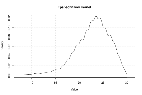
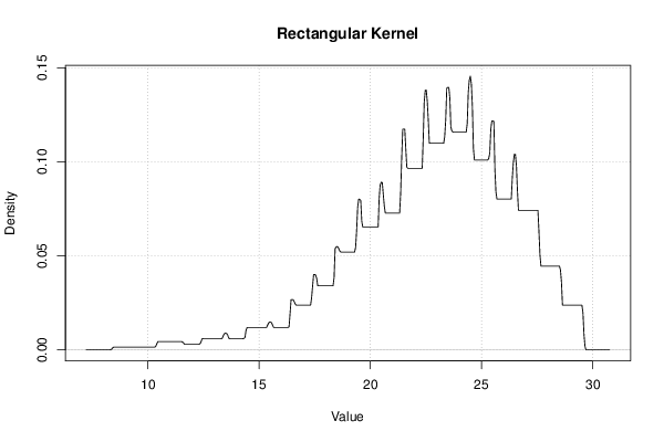
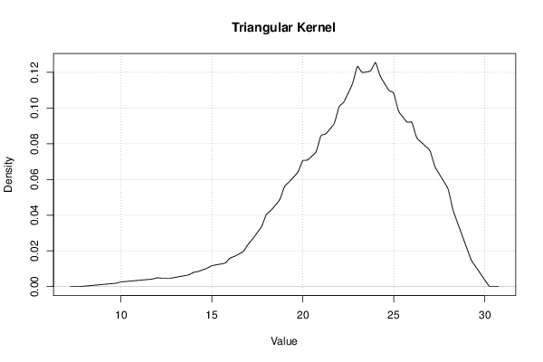
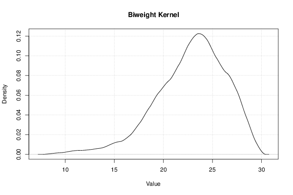
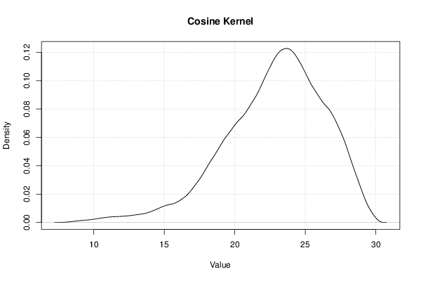
| Title produced by software | Kernel Density Estimation | ||||||||||||||||||||||||||||||||||||||||||||||||||||||||||||||||||||||||||||||||||||||
| Date of computation | Tue, 16 Dec 2014 11:28:10 +0000 | ||||||||||||||||||||||||||||||||||||||||||||||||||||||||||||||||||||||||||||||||||||||
| Cite this page as follows | Statistical Computations at FreeStatistics.org, Office for Research Development and Education, URL https://freestatistics.org/blog/index.php?v=date/2014/Dec/16/t1418729305haxkgfqi2tkis2q.htm/, Retrieved Thu, 16 May 2024 07:19:09 +0000 | ||||||||||||||||||||||||||||||||||||||||||||||||||||||||||||||||||||||||||||||||||||||
| Statistical Computations at FreeStatistics.org, Office for Research Development and Education, URL https://freestatistics.org/blog/index.php?pk=269343, Retrieved Thu, 16 May 2024 07:19:09 +0000 | |||||||||||||||||||||||||||||||||||||||||||||||||||||||||||||||||||||||||||||||||||||||
| QR Codes: | |||||||||||||||||||||||||||||||||||||||||||||||||||||||||||||||||||||||||||||||||||||||
|
| |||||||||||||||||||||||||||||||||||||||||||||||||||||||||||||||||||||||||||||||||||||||
| Original text written by user: | |||||||||||||||||||||||||||||||||||||||||||||||||||||||||||||||||||||||||||||||||||||||
| IsPrivate? | No (this computation is public) | ||||||||||||||||||||||||||||||||||||||||||||||||||||||||||||||||||||||||||||||||||||||
| User-defined keywords | |||||||||||||||||||||||||||||||||||||||||||||||||||||||||||||||||||||||||||||||||||||||
| Estimated Impact | 103 | ||||||||||||||||||||||||||||||||||||||||||||||||||||||||||||||||||||||||||||||||||||||
Tree of Dependent Computations | |||||||||||||||||||||||||||||||||||||||||||||||||||||||||||||||||||||||||||||||||||||||
| Family? (F = Feedback message, R = changed R code, M = changed R Module, P = changed Parameters, D = changed Data) | |||||||||||||||||||||||||||||||||||||||||||||||||||||||||||||||||||||||||||||||||||||||
| - [Maximum-likelihood Fitting - Normal Distribution] [Intrinsic Motivat...] [2010-10-12 11:57:21] [b98453cac15ba1066b407e146608df68] - RMP [Maximum-likelihood Fitting - Normal Distribution] [] [2014-10-14 18:01:50] [32b17a345b130fdf5cc88718ed94a974] - R P [Maximum-likelihood Fitting - Normal Distribution] [] [2014-10-16 17:18:31] [bcf5edf18529a33bd1494456d2c6cb9a] - R PD [Maximum-likelihood Fitting - Normal Distribution] [] [2014-10-16 17:35:06] [bcf5edf18529a33bd1494456d2c6cb9a] - RMP [Kernel Density Estimation] [] [2014-10-16 17:46:22] [bcf5edf18529a33bd1494456d2c6cb9a] - R D [Kernel Density Estimation] [gauss] [2014-12-16 11:28:10] [69667246dd207ce9acb00bd9a43352d5] [Current] | |||||||||||||||||||||||||||||||||||||||||||||||||||||||||||||||||||||||||||||||||||||||
| Feedback Forum | |||||||||||||||||||||||||||||||||||||||||||||||||||||||||||||||||||||||||||||||||||||||
Post a new message | |||||||||||||||||||||||||||||||||||||||||||||||||||||||||||||||||||||||||||||||||||||||
Dataset | |||||||||||||||||||||||||||||||||||||||||||||||||||||||||||||||||||||||||||||||||||||||
| Dataseries X: | |||||||||||||||||||||||||||||||||||||||||||||||||||||||||||||||||||||||||||||||||||||||
23 16 18 28 26 21 20 21 26 15 16 21 25 22 19 24 24 23 22 27 22 24 26 26 28 20 23 24 23 26 20 20 12 21 28 24 24 24 22 26 23 10 27 24 26 18 22 24 16 23 21 28 19 18 27 17 20 24 24 20 24 25 25 26 25 26 14 19 23 25 23 19 23 24 21 21 24 23 22 21 23 25 17 27 28 24 27 22 23 24 24 26 21 23 18 25 24 27 20 25 23 25 24 23 19 25 28 26 24 25 28 23 15 18 24 27 25 24 26 19 23 21 22 23 23 20 20 25 28 19 21 21 25 18 22 21 21 25 20 22 27 23 25 28 25 24 27 19 24 22 23 21 21 20 26 28 23 19 23 18 21 28 22 28 20 23 25 16 23 18 22 21 19 20 27 27 20 26 25 23 24 27 28 26 27 23 28 22 23 27 18 22 23 25 14 21 26 28 22 24 28 24 26 18 19 26 26 12 24 26 23 | |||||||||||||||||||||||||||||||||||||||||||||||||||||||||||||||||||||||||||||||||||||||
Tables (Output of Computation) | |||||||||||||||||||||||||||||||||||||||||||||||||||||||||||||||||||||||||||||||||||||||
| |||||||||||||||||||||||||||||||||||||||||||||||||||||||||||||||||||||||||||||||||||||||
Figures (Output of Computation) | |||||||||||||||||||||||||||||||||||||||||||||||||||||||||||||||||||||||||||||||||||||||
Input Parameters & R Code | |||||||||||||||||||||||||||||||||||||||||||||||||||||||||||||||||||||||||||||||||||||||
| Parameters (Session): | |||||||||||||||||||||||||||||||||||||||||||||||||||||||||||||||||||||||||||||||||||||||
| par1 = 0 ; par2 = no ; par3 = 512 ; | |||||||||||||||||||||||||||||||||||||||||||||||||||||||||||||||||||||||||||||||||||||||
| Parameters (R input): | |||||||||||||||||||||||||||||||||||||||||||||||||||||||||||||||||||||||||||||||||||||||
| par1 = 0 ; par2 = no ; par3 = 512 ; | |||||||||||||||||||||||||||||||||||||||||||||||||||||||||||||||||||||||||||||||||||||||
| R code (references can be found in the software module): | |||||||||||||||||||||||||||||||||||||||||||||||||||||||||||||||||||||||||||||||||||||||
if (par1 == '0') bw <- 'nrd0' | |||||||||||||||||||||||||||||||||||||||||||||||||||||||||||||||||||||||||||||||||||||||