Free Statistics
of Irreproducible Research!
Description of Statistical Computation | |||||||||||||||||||||||||||||||||
|---|---|---|---|---|---|---|---|---|---|---|---|---|---|---|---|---|---|---|---|---|---|---|---|---|---|---|---|---|---|---|---|---|---|
| Author's title | |||||||||||||||||||||||||||||||||
| Author | *The author of this computation has been verified* | ||||||||||||||||||||||||||||||||
| R Software Module | rwasp_meanversusmedian.wasp | ||||||||||||||||||||||||||||||||
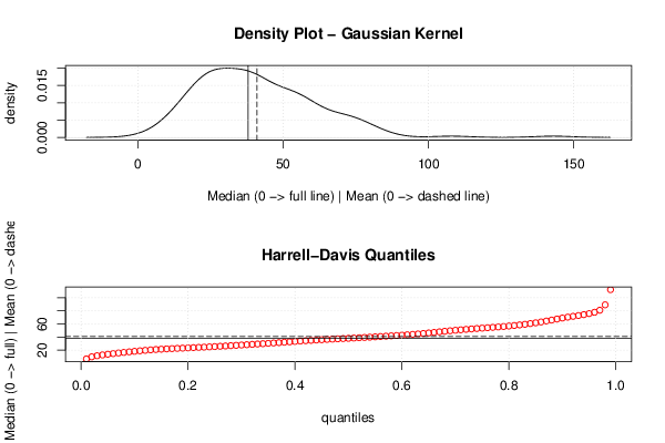
| Title produced by software | Mean versus Median | ||||||||||||||||||||||||||||||||
| Date of computation | Tue, 16 Dec 2014 13:59:14 +0000 | ||||||||||||||||||||||||||||||||
| Cite this page as follows | Statistical Computations at FreeStatistics.org, Office for Research Development and Education, URL https://freestatistics.org/blog/index.php?v=date/2014/Dec/16/t1418738408wj6ywwn60yqpsla.htm/, Retrieved Thu, 16 May 2024 16:45:45 +0000 | ||||||||||||||||||||||||||||||||
| Statistical Computations at FreeStatistics.org, Office for Research Development and Education, URL https://freestatistics.org/blog/index.php?pk=269575, Retrieved Thu, 16 May 2024 16:45:45 +0000 | |||||||||||||||||||||||||||||||||
| QR Codes: | |||||||||||||||||||||||||||||||||
|
| |||||||||||||||||||||||||||||||||
| Original text written by user: | |||||||||||||||||||||||||||||||||
| IsPrivate? | No (this computation is public) | ||||||||||||||||||||||||||||||||
| User-defined keywords | |||||||||||||||||||||||||||||||||
| Estimated Impact | 72 | ||||||||||||||||||||||||||||||||
Tree of Dependent Computations | |||||||||||||||||||||||||||||||||
| Family? (F = Feedback message, R = changed R code, M = changed R Module, P = changed Parameters, D = changed Data) | |||||||||||||||||||||||||||||||||
| - [Two-Way ANOVA] [] [2010-11-02 14:42:14] [b98453cac15ba1066b407e146608df68] - RMP [Two-Way ANOVA] [] [2014-10-21 08:34:19] [32b17a345b130fdf5cc88718ed94a974] - RMPD [Mean versus Median] [gemiddelde CH paper] [2014-12-16 13:59:14] [ca907db95fc0b179b22bb0898c34dff4] [Current] | |||||||||||||||||||||||||||||||||
| Feedback Forum | |||||||||||||||||||||||||||||||||
Post a new message | |||||||||||||||||||||||||||||||||
Dataset | |||||||||||||||||||||||||||||||||
| Dataseries X: | |||||||||||||||||||||||||||||||||
108 10 66 23 25 56 73 34 72 42 74 16 66 9 41 57 48 51 53 55 51 79 39 55 30 55 22 37 2 38 27 56 25 39 33 43 43 23 44 28 39 23 24 29 78 57 37 27 44 39 51 31 24 30 27 14 28 41 31 74 19 51 51 62 59 24 54 39 16 36 31 31 42 39 25 31 38 31 17 22 55 62 51 49 16 12 45 37 37 68 72 143 9 55 17 37 27 37 58 21 19 78 35 48 27 43 30 25 69 72 13 61 43 22 51 67 36 21 44 45 34 36 72 39 43 80 40 61 23 29 29 54 43 20 61 57 54 36 16 40 27 61 69 34 21 34 34 13 12 51 19 81 42 22 85 25 22 19 45 45 51 24 73 24 61 23 14 54 36 26 30 | |||||||||||||||||||||||||||||||||
Tables (Output of Computation) | |||||||||||||||||||||||||||||||||
| |||||||||||||||||||||||||||||||||
Figures (Output of Computation) | |||||||||||||||||||||||||||||||||
Input Parameters & R Code | |||||||||||||||||||||||||||||||||
| Parameters (Session): | |||||||||||||||||||||||||||||||||
| Parameters (R input): | |||||||||||||||||||||||||||||||||
| R code (references can be found in the software module): | |||||||||||||||||||||||||||||||||
library(Hmisc) | |||||||||||||||||||||||||||||||||