Repository of Reproducible Computations

Free Statistics

of Irreproducible Research!

Author's title

Author

*The author of this computation has been verified*

R Software Module

rwasp_bootstrapplot1.wasp

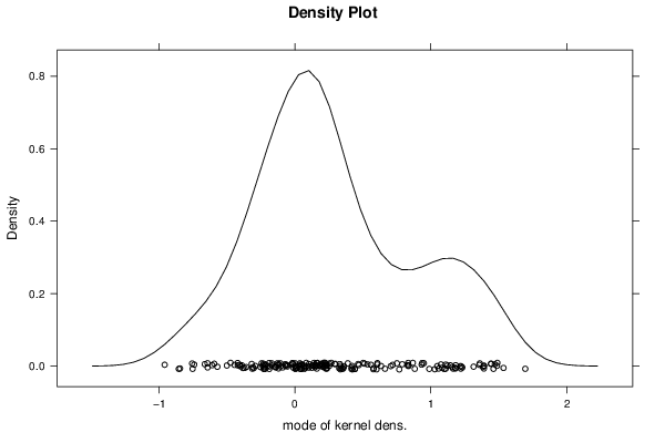
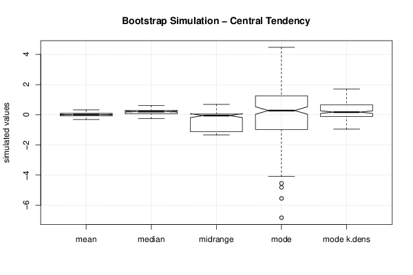
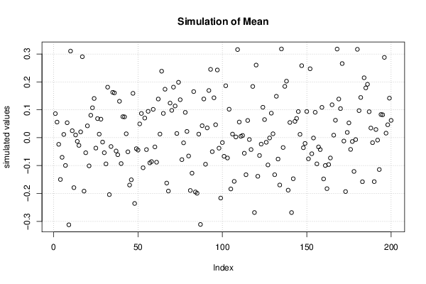
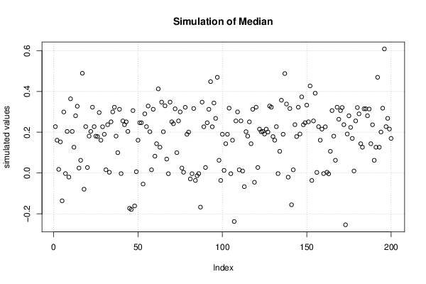
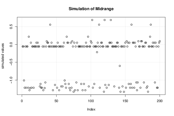
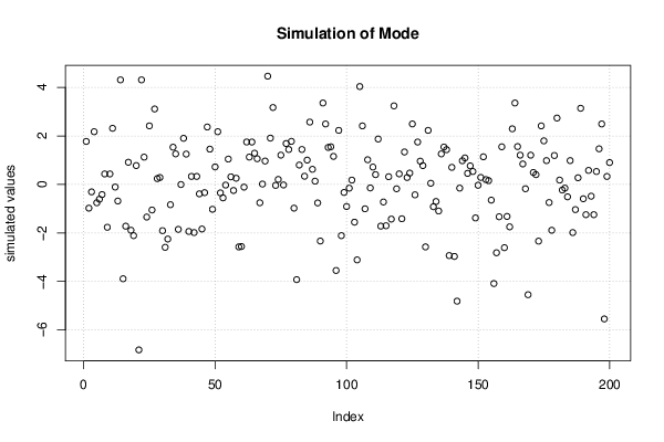
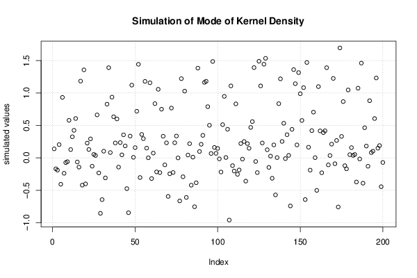
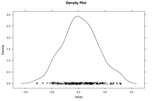
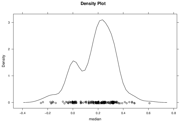
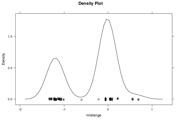
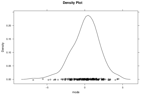
Title produced by software

Bootstrap Plot - Central Tendency

Date of computation

Tue, 16 Dec 2014 14:12:52 +0000

Cite this page as follows

Statistical Computations at FreeStatistics.org, Office for Research Development and Education, URL https://freestatistics.org/blog/index.php?v=date/2014/Dec/16/t1418739180f49gfivtyf3domn.htm/, Retrieved Thu, 16 May 2024 18:53:14 +0000

Statistical Computations at FreeStatistics.org, Office for Research Development and Education, URL https://freestatistics.org/blog/index.php?pk=269594, Retrieved Thu, 16 May 2024 18:53:14 +0000

QR Codes:

Paste this QR Code to cite your computation.

Original text written by user:

IsPrivate?

No (this computation is public)

User-defined keywords

Estimated Impact

Family? (F = Feedback message, R = changed R code, M = changed R Module, P = changed Parameters, D = changed Data)

-     [Bootstrap Plot - Central Tendency] [] [2014-11-04 10:49:59] [32b17a345b130fdf5cc88718ed94a974]
- R  D  [Bootstrap Plot - Central Tendency] [] [2014-11-13 21:57:34] [5efa6717cfe6505454df834acc87b53b]
-    D    [Bootstrap Plot - Central Tendency] [Gemiddelde voorsp...] [2014-12-13 11:35:36] [f12bfb29749f0c3f544bf278d0782c85]
-  M        [Bootstrap Plot - Central Tendency] [Bootstrap] [2014-12-13 11:45:40] [f12bfb29749f0c3f544bf278d0782c85]
-  M            [Bootstrap Plot - Central Tendency] [] [2014-12-16 14:12:52] [24cf8abb2180b57d6cae1ea19168cc61] [Current]

Feedback Forum

Post a new message

Dataseries X:

Download CSV

Histogram

Boxplots

1.05392
-4.38003
1.68564
1.04488
-3.54664
-3.56838
-1.0973
3.11071
4.0352
0.280565
-3.88778
-0.152193
-4.59833
1.44105
-0.388658
-0.661666
1.60859
0.529267
-0.978426
-1.98371
0.389409
-4.23524
3.0134
-3.69722
1.56866
0.753386
-3.41326
3.78982
3.17205
-1.02277
0.329543
-0.42758
-0.127134
-4.4939
-1.10477
-1.41861
1.94621
1.66985
-0.55218
1.77357
-2.49325
-0.00392657
-3.67199
0.50747
1.53499
-0.510477
4.3708
-1.90223
2.84998
-1.34413
3.62441
2.94507
1.1813
-0.494377
0.0862101
0.0158277
3.60471
0.554855
-5.80666
4.34147
0.255476
3.19202
-2.5369
0.467536
-1.45933
2.74868
-3.93889
0.695554
-1.5513
-0.680908
2.17305
1.57027
-0.745077
0.982641
-0.846043
4.46204
-4.08521
2.18738
1.22171
2.10382
1.33694
1.00235
-1.41914
0.126599
2.77974
1.06535
-5.24731
-1.04316
1.55194
2.41307
2.27461
-1.60065
1.56029
3.79709
-4.82802
-1.60367
-1.54846
-2.10759
-2.25947
-3.93671
1.5989
3.79206
-2.19093
2.23945
0.0388132
-0.275799
-1.2289
4.60189
-1.70254
3.42503
-4.89462
-1.86835
-0.775676
0.470672
1.38969
-7.03336
1.40758
2.73662
2.17272
0.532639
-0.440812
-0.755537
2.5338
0.246477
1.04455
2.16284
4.31023
-2.55898
-0.760096
1.33778
0.558967
3.13899
0.597154
0.356976
-0.417547
1.17287
1.4397
0.317868
0.200936
3.04192
-1.50836
2.42324
1.8802
-1.70317
1.84888
0.678294
3.45999
0.227414
0.299637
1.43337
-0.546449
-3.62527
0.178801
-0.0362862
1.54284
-6.48432
1.90048
2.31359
-0.231565
1.33249
-0.17831
2.36712
1.19669
-1.34545
-2.18753
2.22814
2.15755
-0.0539301
6.91914
1.4354
-1.24657
2.29319
0.732644
-0.167038
-2.90493
1.45484
2.35192
-1.87189
-1.02445
-0.976077
3.0202
-0.85838
2.8427
-1.06846
-3.91163
-1.48926
-2.11136
3.35638
0.314765
-3.53653
0.338161
1.74756
-2.57499
-3.6893
0.16091
-2.60733
1.34411
-3.3937
3.04179
-0.513201
0.775836
-1.38094
0.226682
1.00395
0.718173
-0.428344
0.312509
-1.82517
0.0101786
-1.05405
1.20594
-0.553287
-0.155421
-0.590783
3.94099
2.50686
-0.829823
-0.199666
-1.66345
-0.408288
0.203922
-0.786971
1.64101
-1.93625
1.66959
-1.41471
-0.308695
2.4332
-4.59842
-1.82803
1.41813
2.69621
1.96569
1.77455
1.8563
4.37712
3.16089
2.49224
3.4372
-0.561094
-3.11071
-2.63399
-6.82062
-0.79539
-1.15055
-0.00267115
-0.980946
-0.977868
-1.40323
0.426927
1.67856
3.08486
-2.96734
-0.197383
0.907587
-0.0792674
1.09906
-1.11525
-3.15966
-1.00418
0.56347
1.07996
-3.1862
1.13856
-4.811
-5.54416
-2.33365
-6.73701
-1.65842
-2.25021
-4.01845
0.425341
1.81175
0.327383
-0.307673
0.964105
1.4683
-1.54955
-0.144858
-0.965705
1.42259
2.19891
0.618957
-0.361793
0.850687
-3.42402

Summary of computational transaction
Raw Input	view raw input (R code)
Raw Output	view raw output of R engine
Computing time	6 seconds
R Server	'George Udny Yule' @ yule.wessa.net

\begin{tabular}{lllllllll}
\hline
Summary of computational transaction \tabularnewline
Raw Input & view raw input (R code)  \tabularnewline
Raw Output & view raw output of R engine  \tabularnewline
Computing time & 6 seconds \tabularnewline
R Server & 'George Udny Yule' @ yule.wessa.net \tabularnewline
\hline
\end{tabular}
%Source: https://freestatistics.org/blog/index.php?pk=269594&T=0

[TABLE]
[ROW][C]Summary of computational transaction[/C][/ROW]
[ROW][C]Raw Input[/C][C]view raw input (R code) [/C][/ROW]
[ROW][C]Raw Output[/C][C]view raw output of R engine [/C][/ROW]
[ROW][C]Computing time[/C][C]6 seconds[/C][/ROW]
[ROW][C]R Server[/C][C]'George Udny Yule' @ yule.wessa.net[/C][/ROW]
[/TABLE]
Source: https://freestatistics.org/blog/index.php?pk=269594&T=0

Globally Unique Identifier (entire table): ba.freestatistics.org/blog/index.php?pk=269594&T=0

As an alternative you can also use a QR Code:

The GUIDs for individual cells are displayed in the table below:

Summary of computational transaction
Raw Input	view raw input (R code)
Raw Output	view raw output of R engine
Computing time	6 seconds
R Server	'George Udny Yule' @ yule.wessa.net

Estimation Results of Bootstrap
statistic	P1	P5	Q1	Estimate	Q3	P95	P99	S.D.	IQR
mean	-0.2688	-0.19157	-0.072714	6.7063e-08	0.09728	0.24759	0.3167	0.13251	0.16999
median	-0.1789	-0.054564	0.06692	0.20243	0.29721	0.36426	0.48752	0.14823	0.23029
midrange	-1.3281	-1.2857	-1.1164	-0.05711	0.04926	0.21741	0.68749	0.58917	1.1657
mode	-4.8183	-2.9332	-0.97801	6.7063e-08	1.2531	2.7553	4.3102	1.8328	2.2311
mode k.dens	-0.84599	-0.59493	-0.11997	0.1941	0.641	1.3905	1.49	0.58414	0.76098

\begin{tabular}{lllllllll}
\hline
Estimation Results of Bootstrap \tabularnewline
statistic & P1 & P5 & Q1 & Estimate & Q3 & P95 & P99 & S.D. & IQR \tabularnewline
mean & -0.2688 & -0.19157 & -0.072714 & 6.7063e-08 & 0.09728 & 0.24759 & 0.3167 & 0.13251 & 0.16999 \tabularnewline
median & -0.1789 & -0.054564 & 0.06692 & 0.20243 & 0.29721 & 0.36426 & 0.48752 & 0.14823 & 0.23029 \tabularnewline
midrange & -1.3281 & -1.2857 & -1.1164 & -0.05711 & 0.04926 & 0.21741 & 0.68749 & 0.58917 & 1.1657 \tabularnewline
mode & -4.8183 & -2.9332 & -0.97801 & 6.7063e-08 & 1.2531 & 2.7553 & 4.3102 & 1.8328 & 2.2311 \tabularnewline
mode k.dens & -0.84599 & -0.59493 & -0.11997 & 0.1941 & 0.641 & 1.3905 & 1.49 & 0.58414 & 0.76098 \tabularnewline
\hline
\end{tabular}
%Source: https://freestatistics.org/blog/index.php?pk=269594&T=1

[TABLE]
[ROW][C]Estimation Results of Bootstrap[/C][/ROW]
[ROW][C]statistic[/C][C]P1[/C][C]P5[/C][C]Q1[/C][C]Estimate[/C][C]Q3[/C][C]P95[/C][C]P99[/C][C]S.D.[/C][C]IQR[/C][/ROW]
[ROW][C]mean[/C][C]-0.2688[/C][C]-0.19157[/C][C]-0.072714[/C][C]6.7063e-08[/C][C]0.09728[/C][C]0.24759[/C][C]0.3167[/C][C]0.13251[/C][C]0.16999[/C][/ROW]
[ROW][C]median[/C][C]-0.1789[/C][C]-0.054564[/C][C]0.06692[/C][C]0.20243[/C][C]0.29721[/C][C]0.36426[/C][C]0.48752[/C][C]0.14823[/C][C]0.23029[/C][/ROW]
[ROW][C]midrange[/C][C]-1.3281[/C][C]-1.2857[/C][C]-1.1164[/C][C]-0.05711[/C][C]0.04926[/C][C]0.21741[/C][C]0.68749[/C][C]0.58917[/C][C]1.1657[/C][/ROW]
[ROW][C]mode[/C][C]-4.8183[/C][C]-2.9332[/C][C]-0.97801[/C][C]6.7063e-08[/C][C]1.2531[/C][C]2.7553[/C][C]4.3102[/C][C]1.8328[/C][C]2.2311[/C][/ROW]
[ROW][C]mode k.dens[/C][C]-0.84599[/C][C]-0.59493[/C][C]-0.11997[/C][C]0.1941[/C][C]0.641[/C][C]1.3905[/C][C]1.49[/C][C]0.58414[/C][C]0.76098[/C][/ROW]
[/TABLE]
Source: https://freestatistics.org/blog/index.php?pk=269594&T=1

Globally Unique Identifier (entire table): ba.freestatistics.org/blog/index.php?pk=269594&T=1

As an alternative you can also use a QR Code:

The GUIDs for individual cells are displayed in the table below:

Estimation Results of Bootstrap
statistic	P1	P5	Q1	Estimate	Q3	P95	P99	S.D.	IQR
mean	-0.2688	-0.19157	-0.072714	6.7063e-08	0.09728	0.24759	0.3167	0.13251	0.16999
median	-0.1789	-0.054564	0.06692	0.20243	0.29721	0.36426	0.48752	0.14823	0.23029
midrange	-1.3281	-1.2857	-1.1164	-0.05711	0.04926	0.21741	0.68749	0.58917	1.1657
mode	-4.8183	-2.9332	-0.97801	6.7063e-08	1.2531	2.7553	4.3102	1.8328	2.2311
mode k.dens	-0.84599	-0.59493	-0.11997	0.1941	0.641	1.3905	1.49	0.58414	0.76098

Figure 1

PNG link

Postscript link

PDF link

Figure 2

PNG link

Postscript link

PDF link

Figure 3

PNG link

Postscript link

PDF link

Figure 4

PNG link

Postscript link

PDF link

Figure 5

PNG link

Postscript link

PDF link

Figure 6

PNG link

Postscript link

PDF link

Figure 7

PNG link

Postscript link

PDF link

Figure 8

PNG link

Postscript link

PDF link

Figure 9

PNG link

Postscript link

PDF link

Figure 10

PNG link

Postscript link

PDF link

Figure 11

PNG link

Postscript link

PDF link

Parameters (Session):

par1 = 200 ; par2 = 5 ; par3 = 0 ; par4 = P1 P5 Q1 Q3 P95 P99 ;

Parameters (R input):

par1 = 200 ; par2 = 5 ; par3 = 0 ; par4 = P1 P5 Q1 Q3 P95 P99 ;

R code (references can be found in the software module):

par1 <- as.numeric(par1)
par2 <- as.numeric(par2)
if (par3 == '0') bw <- NULL
if (par3 != '0') bw <- as.numeric(par3)
if (par1 < 10) par1 = 10
if (par1 > 5000) par1 = 5000
library(modeest)
library(lattice)
library(boot)
boot.stat <- function(s,i)
{
s.mean <- mean(s[i])
s.median <- median(s[i])
s.midrange <- (max(s[i]) + min(s[i])) / 2
s.mode <- mlv(s[i], method='mfv')$M
s.kernelmode <- mlv(s[i], method='kernel', bw=bw)$M
c(s.mean, s.median, s.midrange, s.mode, s.kernelmode)
}
(r <- boot(x,boot.stat, R=par1, stype='i'))
bitmap(file='plot1.png')
plot(r$t[,1],type='p',ylab='simulated values',main='Simulation of Mean')
grid()
dev.off()
bitmap(file='plot2.png')
plot(r$t[,2],type='p',ylab='simulated values',main='Simulation of Median')
grid()
dev.off()
bitmap(file='plot3.png')
plot(r$t[,3],type='p',ylab='simulated values',main='Simulation of Midrange')
grid()
dev.off()
bitmap(file='plot7.png')
plot(r$t[,4],type='p',ylab='simulated values',main='Simulation of Mode')
grid()
dev.off()
bitmap(file='plot8.png')
plot(r$t[,5],type='p',ylab='simulated values',main='Simulation of Mode of Kernel Density')
grid()
dev.off()
bitmap(file='plot4.png')
densityplot(~r$t[,1],col='black',main='Density Plot',xlab='mean')
dev.off()
bitmap(file='plot5.png')
densityplot(~r$t[,2],col='black',main='Density Plot',xlab='median')
dev.off()
bitmap(file='plot6.png')
densityplot(~r$t[,3],col='black',main='Density Plot',xlab='midrange')
dev.off()
bitmap(file='plot9.png')
densityplot(~r$t[,4],col='black',main='Density Plot',xlab='mode')
dev.off()
bitmap(file='plot10.png')
densityplot(~r$t[,5],col='black',main='Density Plot',xlab='mode of kernel dens.')
dev.off()
z <- data.frame(cbind(r$t[,1],r$t[,2],r$t[,3],r$t[,4],r$t[,5]))
colnames(z) <- list('mean','median','midrange','mode','mode k.dens')
bitmap(file='plot11.png')
boxplot(z,notch=TRUE,ylab='simulated values',main='Bootstrap Simulation - Central Tendency')
grid()
dev.off()
load(file='createtable')
a<-table.start()
a<-table.row.start(a)
a<-table.element(a,'Estimation Results of Bootstrap',10,TRUE)
a<-table.row.end(a)
if (par4 == 'P1 P5 Q1 Q3 P95 P99') {
myq.1 <- 0.01
myq.2 <- 0.05
myq.3 <- 0.95
myq.4 <- 0.99
myl.1 <- 'P1'
myl.2 <- 'P5'
myl.3 <- 'P95'
myl.4 <- 'P99'
}
if (par4 == 'P0.5 P2.5 Q1 Q3 P97.5 P99.5') {
myq.1 <- 0.005
myq.2 <- 0.025
myq.3 <- 0.975
myq.4 <- 0.995
myl.1 <- 'P0.5'
myl.2 <- 'P2.5'
myl.3 <- 'P97.5'
myl.4 <- 'P99.5'
}
if (par4 == 'P10 P20 Q1 Q3 P80 P90') {
myq.1 <- 0.10
myq.2 <- 0.20
myq.3 <- 0.80
myq.4 <- 0.90
myl.1 <- 'P10'
myl.2 <- 'P20'
myl.3 <- 'P80'
myl.4 <- 'P90'
}
a<-table.row.start(a)
a<-table.element(a,'statistic',header=TRUE)
a<-table.element(a,myl.1,header=TRUE)
a<-table.element(a,myl.2,header=TRUE)
a<-table.element(a,'Q1',header=TRUE)
a<-table.element(a,'Estimate',header=TRUE)
a<-table.element(a,'Q3',header=TRUE)
a<-table.element(a,myl.3,header=TRUE)
a<-table.element(a,myl.4,header=TRUE)
a<-table.element(a,'S.D.',header=TRUE)
a<-table.element(a,'IQR',header=TRUE)
a<-table.row.end(a)
a<-table.row.start(a)
a<-table.element(a,'mean',header=TRUE)
q1 <- quantile(r$t[,1],0.25)[[1]]
q3 <- quantile(r$t[,1],0.75)[[1]]
p01 <- quantile(r$t[,1],myq.1)[[1]]
p05 <- quantile(r$t[,1],myq.2)[[1]]
p95 <- quantile(r$t[,1],myq.3)[[1]]
p99 <- quantile(r$t[,1],myq.4)[[1]]
a<-table.element(a,signif(p01,par2))
a<-table.element(a,signif(p05,par2))
a<-table.element(a,signif(q1,par2))
a<-table.element(a,signif(r$t0[1],par2))
a<-table.element(a,signif(q3,par2))
a<-table.element(a,signif(p95,par2))
a<-table.element(a,signif(p99,par2))
a<-table.element( a,signif( sqrt(var(r$t[,1])),par2 ) )
a<-table.element(a,signif(q3-q1,par2))
a<-table.row.end(a)
a<-table.row.start(a)
a<-table.element(a,'median',header=TRUE)
q1 <- quantile(r$t[,2],0.25)[[1]]
q3 <- quantile(r$t[,2],0.75)[[1]]
p01 <- quantile(r$t[,2],myq.1)[[1]]
p05 <- quantile(r$t[,2],myq.2)[[1]]
p95 <- quantile(r$t[,2],myq.3)[[1]]
p99 <- quantile(r$t[,2],myq.4)[[1]]
a<-table.element(a,signif(p01,par2))
a<-table.element(a,signif(p05,par2))
a<-table.element(a,signif(q1,par2))
a<-table.element(a,signif(r$t0[2],par2))
a<-table.element(a,signif(q3,par2))
a<-table.element(a,signif(p95,par2))
a<-table.element(a,signif(p99,par2))
a<-table.element(a,signif(sqrt(var(r$t[,2])),par2))
a<-table.element(a,signif(q3-q1,par2))
a<-table.row.end(a)
a<-table.row.start(a)
a<-table.element(a,'midrange',header=TRUE)
q1 <- quantile(r$t[,3],0.25)[[1]]
q3 <- quantile(r$t[,3],0.75)[[1]]
p01 <- quantile(r$t[,3],myq.1)[[1]]
p05 <- quantile(r$t[,3],myq.2)[[1]]
p95 <- quantile(r$t[,3],myq.3)[[1]]
p99 <- quantile(r$t[,3],myq.4)[[1]]
a<-table.element(a,signif(p01,par2))
a<-table.element(a,signif(p05,par2))
a<-table.element(a,signif(q1,par2))
a<-table.element(a,signif(r$t0[3],par2))
a<-table.element(a,signif(q3,par2))
a<-table.element(a,signif(p95,par2))
a<-table.element(a,signif(p99,par2))
a<-table.element(a,signif(sqrt(var(r$t[,3])),par2))
a<-table.element(a,signif(q3-q1,par2))
a<-table.row.end(a)
a<-table.row.start(a)
a<-table.element(a,'mode',header=TRUE)
q1 <- quantile(r$t[,4],0.25)[[1]]
q3 <- quantile(r$t[,4],0.75)[[1]]
p01 <- quantile(r$t[,4],myq.1)[[1]]
p05 <- quantile(r$t[,4],myq.2)[[1]]
p95 <- quantile(r$t[,4],myq.3)[[1]]
p99 <- quantile(r$t[,4],myq.4)[[1]]
a<-table.element(a,signif(p01,par2))
a<-table.element(a,signif(p05,par2))
a<-table.element(a,signif(q1,par2))
a<-table.element(a,signif(r$t0[4],par2))
a<-table.element(a,signif(q3,par2))
a<-table.element(a,signif(p95,par2))
a<-table.element(a,signif(p99,par2))
a<-table.element(a,signif(sqrt(var(r$t[,4])),par2))
a<-table.element(a,signif(q3-q1,par2))
a<-table.row.end(a)
a<-table.row.start(a)
a<-table.element(a,'mode k.dens',header=TRUE)
q1 <- quantile(r$t[,5],0.25)[[1]]
q3 <- quantile(r$t[,5],0.75)[[1]]
p01 <- quantile(r$t[,5],myq.1)[[1]]
p05 <- quantile(r$t[,5],myq.2)[[1]]
p95 <- quantile(r$t[,5],myq.3)[[1]]
p99 <- quantile(r$t[,5],myq.4)[[1]]
a<-table.element(a,signif(p01,par2))
a<-table.element(a,signif(p05,par2))
a<-table.element(a,signif(q1,par2))
a<-table.element(a,signif(r$t0[5],par2))
a<-table.element(a,signif(q3,par2))
a<-table.element(a,signif(p95,par2))
a<-table.element(a,signif(p99,par2))
a<-table.element(a,signif(sqrt(var(r$t[,5])),par2))
a<-table.element(a,signif(q3-q1,par2))
a<-table.row.end(a)
a<-table.end(a)
table.save(a,file='mytable.tab')

Free Statistics

Description of Statistical Computation

Tree of Dependent Computations

Dataset

Tables (Output of Computation)

Figures (Output of Computation)

Input Parameters & R Code