Free Statistics
of Irreproducible Research!
Description of Statistical Computation | |||||||||||||||||||||||||||||||||||||||||||||||||||||||||||||||||||||||||||||||||
|---|---|---|---|---|---|---|---|---|---|---|---|---|---|---|---|---|---|---|---|---|---|---|---|---|---|---|---|---|---|---|---|---|---|---|---|---|---|---|---|---|---|---|---|---|---|---|---|---|---|---|---|---|---|---|---|---|---|---|---|---|---|---|---|---|---|---|---|---|---|---|---|---|---|---|---|---|---|---|---|---|---|
| Author's title | |||||||||||||||||||||||||||||||||||||||||||||||||||||||||||||||||||||||||||||||||
| Author | *The author of this computation has been verified* | ||||||||||||||||||||||||||||||||||||||||||||||||||||||||||||||||||||||||||||||||
| R Software Module | rwasp_notchedbox1.wasp | ||||||||||||||||||||||||||||||||||||||||||||||||||||||||||||||||||||||||||||||||
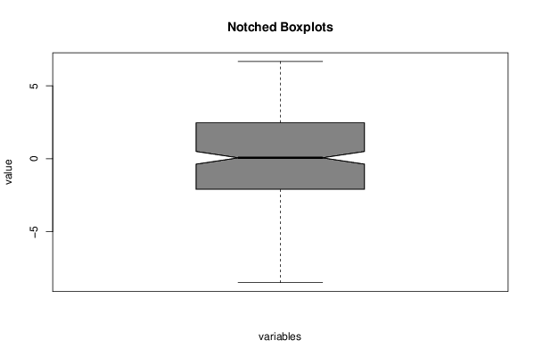
| Title produced by software | Notched Boxplots | ||||||||||||||||||||||||||||||||||||||||||||||||||||||||||||||||||||||||||||||||
| Date of computation | Wed, 17 Dec 2014 11:49:30 +0000 | ||||||||||||||||||||||||||||||||||||||||||||||||||||||||||||||||||||||||||||||||
| Cite this page as follows | Statistical Computations at FreeStatistics.org, Office for Research Development and Education, URL https://freestatistics.org/blog/index.php?v=date/2014/Dec/17/t1418817015blkhl00mcbrt9xn.htm/, Retrieved Thu, 16 May 2024 21:59:14 +0000 | ||||||||||||||||||||||||||||||||||||||||||||||||||||||||||||||||||||||||||||||||
| Statistical Computations at FreeStatistics.org, Office for Research Development and Education, URL https://freestatistics.org/blog/index.php?pk=270071, Retrieved Thu, 16 May 2024 21:59:14 +0000 | |||||||||||||||||||||||||||||||||||||||||||||||||||||||||||||||||||||||||||||||||
| QR Codes: | |||||||||||||||||||||||||||||||||||||||||||||||||||||||||||||||||||||||||||||||||
|
| |||||||||||||||||||||||||||||||||||||||||||||||||||||||||||||||||||||||||||||||||
| Original text written by user: | |||||||||||||||||||||||||||||||||||||||||||||||||||||||||||||||||||||||||||||||||
| IsPrivate? | No (this computation is public) | ||||||||||||||||||||||||||||||||||||||||||||||||||||||||||||||||||||||||||||||||
| User-defined keywords | |||||||||||||||||||||||||||||||||||||||||||||||||||||||||||||||||||||||||||||||||
| Estimated Impact | 51 | ||||||||||||||||||||||||||||||||||||||||||||||||||||||||||||||||||||||||||||||||
Tree of Dependent Computations | |||||||||||||||||||||||||||||||||||||||||||||||||||||||||||||||||||||||||||||||||
| Family? (F = Feedback message, R = changed R code, M = changed R Module, P = changed Parameters, D = changed Data) | |||||||||||||||||||||||||||||||||||||||||||||||||||||||||||||||||||||||||||||||||
| - [Notched Boxplots] [] [2014-12-17 11:49:30] [1f9cde3fd5a46d58696c891290fd755a] [Current] | |||||||||||||||||||||||||||||||||||||||||||||||||||||||||||||||||||||||||||||||||
| Feedback Forum | |||||||||||||||||||||||||||||||||||||||||||||||||||||||||||||||||||||||||||||||||
Post a new message | |||||||||||||||||||||||||||||||||||||||||||||||||||||||||||||||||||||||||||||||||
Dataset | |||||||||||||||||||||||||||||||||||||||||||||||||||||||||||||||||||||||||||||||||
| Dataseries X: | |||||||||||||||||||||||||||||||||||||||||||||||||||||||||||||||||||||||||||||||||
-0.886662 -0.636593 -0.986662 -5.43659 -6.13659 -0.236593 1.01334 0.463407 -1.73659 -4.63659 -1.43659 -6.43659 -2.23659 -1.78666 -7.48666 -1.93129 -0.936593 -4.48666 -2.68122 -3.78666 -6.43659 0.963407 -2.98666 0.963407 -1.13659 -1.93659 3.81878 0.168714 -2.93659 -2.28666 -5.48666 -2.08666 -3.83659 -3.13659 -2.03659 -2.53659 -3.38666 0.418783 -3.53659 -1.98666 -6.93659 -1.43659 0.163407 -2.03659 0.018783 -2.48666 -1.03659 -4.38122 -1.08666 0.018783 -0.681217 -5.58122 -1.93659 -0.181217 0.463407 -2.73659 -7.53129 1.46341 -5.23129 1.01878 -3.53659 -1.28666 -6.18666 3.06341 -4.58666 -3.18122 -2.68666 0.163407 1.66341 -1.03129 -1.48666 -2.38666 -4.43129 2.31878 -1.18666 -0.786662 0.318783 -0.586662 -3.33129 -5.13659 -2.73129 0.168714 -2.33129 -7.98122 -2.93129 -0.481217 -1.08122 -1.83129 -4.63129 -0.031286 0.318783 -6.68122 -2.38122 -4.43129 -4.58122 -4.23129 -4.98122 -0.881217 1.31878 -4.38122 -1.58122 -2.93129 -3.98122 -2.68122 1.91878 -4.73129 0.268714 -8.33129 -6.83129 -3.63129 -1.63129 -1.18122 -8.48659 -0.136593 5.26341 5.01341 3.36871 0.318783 4.26341 5.31334 3.26341 -0.436662 4.61334 1.86341 -2.23659 -0.236593 3.36341 0.763407 6.61878 1.26341 1.66341 2.36334 1.91341 1.96341 -0.386593 -0.186593 4.51341 -4.23659 4.61334 3.26341 -0.681217 4.91341 2.41341 4.81341 2.56334 3.86334 0.763407 0.563338 0.963338 5.41341 -3.88666 3.16341 5.41341 3.06334 2.31878 1.56878 6.11341 1.81334 1.61871 -1.48129 5.21871 3.61878 3.31334 3.26341 6.66871 -1.33122 5.21871 2.81878 1.76871 -1.88129 3.66878 4.86871 2.31878 2.56341 2.56341 5.31878 0.513407 5.31334 3.06878 -6.18666 0.168714 0.668714 6.26341 2.01871 0.618783 2.86871 4.11871 -0.081286 -1.08129 0.318783 -1.93122 3.11878 -2.68122 4.96871 0.368714 2.56878 0.963338 0.868714 1.66871 3.01871 6.41341 1.31878 -0.186662 2.41871 -0.086593 1.36871 -2.98659 0.368783 5.96871 4.31878 -1.08122 2.41341 -1.88666 -0.031286 2.56334 -0.436593 3.56878 5.31341 -1.13122 2.41871 3.96334 -5.58129 -0.486593 2.76341 5.51334 1.96871 3.31334 3.31878 5.56341 5.26334 4.76334 5.31334 0.818783 0.013407 -3.33659 -8.33659 -1.38129 0.763407 -1.13659 0.118783 -0.436662 -1.83129 2.61878 6.66871 -1.08122 2.31878 3.81334 1.21341 2.31334 0.513407 -0.986593 -1.83666 2.46878 1.91871 0.363407 3.61871 -4.43122 -6.08666 -0.631286 -4.43122 -1.33122 -0.881286 -2.33122 2.61878 3.41871 1.11878 0.718714 2.46871 4.56878 -1.33122 2.11871 -0.081217 1.86871 4.51871 2.91878 0.813338 3.41871 -4.18122 | |||||||||||||||||||||||||||||||||||||||||||||||||||||||||||||||||||||||||||||||||
Tables (Output of Computation) | |||||||||||||||||||||||||||||||||||||||||||||||||||||||||||||||||||||||||||||||||
| |||||||||||||||||||||||||||||||||||||||||||||||||||||||||||||||||||||||||||||||||
Figures (Output of Computation) | |||||||||||||||||||||||||||||||||||||||||||||||||||||||||||||||||||||||||||||||||
Input Parameters & R Code | |||||||||||||||||||||||||||||||||||||||||||||||||||||||||||||||||||||||||||||||||
| Parameters (Session): | |||||||||||||||||||||||||||||||||||||||||||||||||||||||||||||||||||||||||||||||||
| par1 = grey ; | |||||||||||||||||||||||||||||||||||||||||||||||||||||||||||||||||||||||||||||||||
| Parameters (R input): | |||||||||||||||||||||||||||||||||||||||||||||||||||||||||||||||||||||||||||||||||
| par1 = grey ; | |||||||||||||||||||||||||||||||||||||||||||||||||||||||||||||||||||||||||||||||||
| R code (references can be found in the software module): | |||||||||||||||||||||||||||||||||||||||||||||||||||||||||||||||||||||||||||||||||
z <- as.data.frame(t(y)) | |||||||||||||||||||||||||||||||||||||||||||||||||||||||||||||||||||||||||||||||||