Repository of Reproducible Computations

Free Statistics

of Irreproducible Research!

Author's title

Author

*The author of this computation has been verified*

R Software Module

rwasp_autocorrelation.wasp

Title produced by software

(Partial) Autocorrelation Function

Date of computation

Wed, 17 Dec 2014 14:23:55 +0000

Cite this page as follows

Statistical Computations at FreeStatistics.org, Office for Research Development and Education, URL https://freestatistics.org/blog/index.php?v=date/2014/Dec/17/t1418826273gnoqcvhpn6ndzwe.htm/, Retrieved Thu, 16 May 2024 07:09:06 +0000

Statistical Computations at FreeStatistics.org, Office for Research Development and Education, URL https://freestatistics.org/blog/index.php?pk=270316, Retrieved Thu, 16 May 2024 07:09:06 +0000

QR Codes:

Paste this QR Code to cite your computation.

Original text written by user:

IsPrivate?

No (this computation is public)

User-defined keywords

Estimated Impact

Family? (F = Feedback message, R = changed R code, M = changed R Module, P = changed Parameters, D = changed Data)

-     [Univariate Data Series] [] [2008-12-08 19:22:39] [d2d412c7f4d35ffbf5ee5ee89db327d4]
- RMP   [(Partial) Autocorrelation Function] [] [2011-12-06 19:49:59] [b98453cac15ba1066b407e146608df68]
- RM      [(Partial) Autocorrelation Function] [] [2014-11-26 14:53:44] [bcf5edf18529a33bd1494456d2c6cb9a]
-  MPD        [(Partial) Autocorrelation Function] [] [2014-12-17 14:23:55] [6fc1b517ba5ef695988bbc0a377c4b82] [Current]

Feedback Forum

Post a new message

Dataseries X:

Download CSV

Histogram

Boxplots

Summary of computational transaction
Raw Input	view raw input (R code)
Raw Output	view raw output of R engine
Computing time	1 seconds
R Server	'Gertrude Mary Cox' @ cox.wessa.net

\begin{tabular}{lllllllll}
\hline
Summary of computational transaction \tabularnewline
Raw Input & view raw input (R code)  \tabularnewline
Raw Output & view raw output of R engine  \tabularnewline
Computing time & 1 seconds \tabularnewline
R Server & 'Gertrude Mary Cox' @ cox.wessa.net \tabularnewline
\hline
\end{tabular}
%Source: https://freestatistics.org/blog/index.php?pk=270316&T=0

[TABLE]
[ROW][C]Summary of computational transaction[/C][/ROW]
[ROW][C]Raw Input[/C][C]view raw input (R code) [/C][/ROW]
[ROW][C]Raw Output[/C][C]view raw output of R engine [/C][/ROW]
[ROW][C]Computing time[/C][C]1 seconds[/C][/ROW]
[ROW][C]R Server[/C][C]'Gertrude Mary Cox' @ cox.wessa.net[/C][/ROW]
[/TABLE]
Source: https://freestatistics.org/blog/index.php?pk=270316&T=0

Globally Unique Identifier (entire table): ba.freestatistics.org/blog/index.php?pk=270316&T=0

As an alternative you can also use a QR Code:

The GUIDs for individual cells are displayed in the table below:

Summary of computational transaction
Raw Input	view raw input (R code)
Raw Output	view raw output of R engine
Computing time	1 seconds
R Server	'Gertrude Mary Cox' @ cox.wessa.net

Autocorrelation Function
Time lag k	ACF(k)	T-STAT	P-value
1	0.360866	6.1028	0
2	0.347141	5.8707	0
3	0.351638	5.9467	0
4	0.341277	5.7715	0
5	0.338835	5.7302	0
6	0.234998	3.9742	4.5e-05
7	0.235275	3.9789	4.4e-05
8	0.237587	4.018	3.8e-05
9	0.26662	4.509	5e-06
10	0.268576	4.542	4e-06
11	0.255358	4.3185	1.1e-05
12	0.277698	4.6963	2e-06
13	0.283127	4.7881	1e-06
14	0.235289	3.9791	4.4e-05
15	0.241013	4.0759	3e-05
16	0.286928	4.8524	1e-06
17	0.246523	4.1691	2e-05
18	0.267297	4.5204	5e-06
19	0.256388	4.3359	1e-05
20	0.234735	3.9697	4.6e-05
21	0.217578	3.6796	0.00014
22	0.265632	4.4922	5e-06
23	0.249016	4.2112	1.7e-05
24	0.265473	4.4896	5e-06
25	0.255887	4.3274	1e-05
26	0.18111	3.0628	0.001201
27	0.208415	3.5246	0.000247
28	0.214969	3.6355	0.000164
29	0.219848	3.718	0.000121
30	0.19811	3.3503	0.000458
31	0.117741	1.9912	0.023706
32	0.185356	3.1347	0.00095
33	0.189811	3.21	0.000739
34	0.149555	2.5292	0.005985
35	0.105113	1.7776	0.038265
36	0.137991	2.3336	0.010154

\begin{tabular}{lllllllll}
\hline
Autocorrelation Function \tabularnewline
Time lag k & ACF(k) & T-STAT & P-value \tabularnewline
1 & 0.360866 & 6.1028 & 0 \tabularnewline
2 & 0.347141 & 5.8707 & 0 \tabularnewline
3 & 0.351638 & 5.9467 & 0 \tabularnewline
4 & 0.341277 & 5.7715 & 0 \tabularnewline
5 & 0.338835 & 5.7302 & 0 \tabularnewline
6 & 0.234998 & 3.9742 & 4.5e-05 \tabularnewline
7 & 0.235275 & 3.9789 & 4.4e-05 \tabularnewline
8 & 0.237587 & 4.018 & 3.8e-05 \tabularnewline
9 & 0.26662 & 4.509 & 5e-06 \tabularnewline
10 & 0.268576 & 4.542 & 4e-06 \tabularnewline
11 & 0.255358 & 4.3185 & 1.1e-05 \tabularnewline
12 & 0.277698 & 4.6963 & 2e-06 \tabularnewline
13 & 0.283127 & 4.7881 & 1e-06 \tabularnewline
14 & 0.235289 & 3.9791 & 4.4e-05 \tabularnewline
15 & 0.241013 & 4.0759 & 3e-05 \tabularnewline
16 & 0.286928 & 4.8524 & 1e-06 \tabularnewline
17 & 0.246523 & 4.1691 & 2e-05 \tabularnewline
18 & 0.267297 & 4.5204 & 5e-06 \tabularnewline
19 & 0.256388 & 4.3359 & 1e-05 \tabularnewline
20 & 0.234735 & 3.9697 & 4.6e-05 \tabularnewline
21 & 0.217578 & 3.6796 & 0.00014 \tabularnewline
22 & 0.265632 & 4.4922 & 5e-06 \tabularnewline
23 & 0.249016 & 4.2112 & 1.7e-05 \tabularnewline
24 & 0.265473 & 4.4896 & 5e-06 \tabularnewline
25 & 0.255887 & 4.3274 & 1e-05 \tabularnewline
26 & 0.18111 & 3.0628 & 0.001201 \tabularnewline
27 & 0.208415 & 3.5246 & 0.000247 \tabularnewline
28 & 0.214969 & 3.6355 & 0.000164 \tabularnewline
29 & 0.219848 & 3.718 & 0.000121 \tabularnewline
30 & 0.19811 & 3.3503 & 0.000458 \tabularnewline
31 & 0.117741 & 1.9912 & 0.023706 \tabularnewline
32 & 0.185356 & 3.1347 & 0.00095 \tabularnewline
33 & 0.189811 & 3.21 & 0.000739 \tabularnewline
34 & 0.149555 & 2.5292 & 0.005985 \tabularnewline
35 & 0.105113 & 1.7776 & 0.038265 \tabularnewline
36 & 0.137991 & 2.3336 & 0.010154 \tabularnewline
\hline
\end{tabular}
%Source: https://freestatistics.org/blog/index.php?pk=270316&T=1

[TABLE]
[ROW][C]Autocorrelation Function[/C][/ROW]
[ROW][C]Time lag k[/C][C]ACF(k)[/C][C]T-STAT[/C][C]P-value[/C][/ROW]
[ROW][C]1[/C][C]0.360866[/C][C]6.1028[/C][C]0[/C][/ROW]
[ROW][C]2[/C][C]0.347141[/C][C]5.8707[/C][C]0[/C][/ROW]
[ROW][C]3[/C][C]0.351638[/C][C]5.9467[/C][C]0[/C][/ROW]
[ROW][C]4[/C][C]0.341277[/C][C]5.7715[/C][C]0[/C][/ROW]
[ROW][C]5[/C][C]0.338835[/C][C]5.7302[/C][C]0[/C][/ROW]
[ROW][C]6[/C][C]0.234998[/C][C]3.9742[/C][C]4.5e-05[/C][/ROW]
[ROW][C]7[/C][C]0.235275[/C][C]3.9789[/C][C]4.4e-05[/C][/ROW]
[ROW][C]8[/C][C]0.237587[/C][C]4.018[/C][C]3.8e-05[/C][/ROW]
[ROW][C]9[/C][C]0.26662[/C][C]4.509[/C][C]5e-06[/C][/ROW]
[ROW][C]10[/C][C]0.268576[/C][C]4.542[/C][C]4e-06[/C][/ROW]
[ROW][C]11[/C][C]0.255358[/C][C]4.3185[/C][C]1.1e-05[/C][/ROW]
[ROW][C]12[/C][C]0.277698[/C][C]4.6963[/C][C]2e-06[/C][/ROW]
[ROW][C]13[/C][C]0.283127[/C][C]4.7881[/C][C]1e-06[/C][/ROW]
[ROW][C]14[/C][C]0.235289[/C][C]3.9791[/C][C]4.4e-05[/C][/ROW]
[ROW][C]15[/C][C]0.241013[/C][C]4.0759[/C][C]3e-05[/C][/ROW]
[ROW][C]16[/C][C]0.286928[/C][C]4.8524[/C][C]1e-06[/C][/ROW]
[ROW][C]17[/C][C]0.246523[/C][C]4.1691[/C][C]2e-05[/C][/ROW]
[ROW][C]18[/C][C]0.267297[/C][C]4.5204[/C][C]5e-06[/C][/ROW]
[ROW][C]19[/C][C]0.256388[/C][C]4.3359[/C][C]1e-05[/C][/ROW]
[ROW][C]20[/C][C]0.234735[/C][C]3.9697[/C][C]4.6e-05[/C][/ROW]
[ROW][C]21[/C][C]0.217578[/C][C]3.6796[/C][C]0.00014[/C][/ROW]
[ROW][C]22[/C][C]0.265632[/C][C]4.4922[/C][C]5e-06[/C][/ROW]
[ROW][C]23[/C][C]0.249016[/C][C]4.2112[/C][C]1.7e-05[/C][/ROW]
[ROW][C]24[/C][C]0.265473[/C][C]4.4896[/C][C]5e-06[/C][/ROW]
[ROW][C]25[/C][C]0.255887[/C][C]4.3274[/C][C]1e-05[/C][/ROW]
[ROW][C]26[/C][C]0.18111[/C][C]3.0628[/C][C]0.001201[/C][/ROW]
[ROW][C]27[/C][C]0.208415[/C][C]3.5246[/C][C]0.000247[/C][/ROW]
[ROW][C]28[/C][C]0.214969[/C][C]3.6355[/C][C]0.000164[/C][/ROW]
[ROW][C]29[/C][C]0.219848[/C][C]3.718[/C][C]0.000121[/C][/ROW]
[ROW][C]30[/C][C]0.19811[/C][C]3.3503[/C][C]0.000458[/C][/ROW]
[ROW][C]31[/C][C]0.117741[/C][C]1.9912[/C][C]0.023706[/C][/ROW]
[ROW][C]32[/C][C]0.185356[/C][C]3.1347[/C][C]0.00095[/C][/ROW]
[ROW][C]33[/C][C]0.189811[/C][C]3.21[/C][C]0.000739[/C][/ROW]
[ROW][C]34[/C][C]0.149555[/C][C]2.5292[/C][C]0.005985[/C][/ROW]
[ROW][C]35[/C][C]0.105113[/C][C]1.7776[/C][C]0.038265[/C][/ROW]
[ROW][C]36[/C][C]0.137991[/C][C]2.3336[/C][C]0.010154[/C][/ROW]
[/TABLE]
Source: https://freestatistics.org/blog/index.php?pk=270316&T=1

Globally Unique Identifier (entire table): ba.freestatistics.org/blog/index.php?pk=270316&T=1

As an alternative you can also use a QR Code:

The GUIDs for individual cells are displayed in the table below:

Autocorrelation Function
Time lag k	ACF(k)	T-STAT	P-value
1	0.360866	6.1028	0
2	0.347141	5.8707	0
3	0.351638	5.9467	0
4	0.341277	5.7715	0
5	0.338835	5.7302	0
6	0.234998	3.9742	4.5e-05
7	0.235275	3.9789	4.4e-05
8	0.237587	4.018	3.8e-05
9	0.26662	4.509	5e-06
10	0.268576	4.542	4e-06
11	0.255358	4.3185	1.1e-05
12	0.277698	4.6963	2e-06
13	0.283127	4.7881	1e-06
14	0.235289	3.9791	4.4e-05
15	0.241013	4.0759	3e-05
16	0.286928	4.8524	1e-06
17	0.246523	4.1691	2e-05
18	0.267297	4.5204	5e-06
19	0.256388	4.3359	1e-05
20	0.234735	3.9697	4.6e-05
21	0.217578	3.6796	0.00014
22	0.265632	4.4922	5e-06
23	0.249016	4.2112	1.7e-05
24	0.265473	4.4896	5e-06
25	0.255887	4.3274	1e-05
26	0.18111	3.0628	0.001201
27	0.208415	3.5246	0.000247
28	0.214969	3.6355	0.000164
29	0.219848	3.718	0.000121
30	0.19811	3.3503	0.000458
31	0.117741	1.9912	0.023706
32	0.185356	3.1347	0.00095
33	0.189811	3.21	0.000739
34	0.149555	2.5292	0.005985
35	0.105113	1.7776	0.038265
36	0.137991	2.3336	0.010154

Partial Autocorrelation Function
Time lag k	PACF(k)	T-STAT	P-value
1	0.360866	6.1028	0
2	0.249394	4.2176	1.7e-05
3	0.205487	3.4751	0.000295
4	0.156986	2.6549	0.004189
5	0.133136	2.2515	0.012555
6	-0.021031	-0.3557	0.361178
7	0.010169	0.172	0.43179
8	0.032531	0.5501	0.291326
9	0.088952	1.5043	0.066803
10	0.088973	1.5047	0.066757
11	0.069016	1.1672	0.122059
12	0.079423	1.3432	0.090141
13	0.065313	1.1045	0.135144
14	-0.016811	-0.2843	0.388195
15	0.009705	0.1641	0.434877
16	0.087004	1.4714	0.071146
17	0.022271	0.3766	0.353359
18	0.062591	1.0585	0.145358
19	0.045427	0.7682	0.221487
20	-0.000811	-0.0137	0.494533
21	-0.030358	-0.5134	0.304036
22	0.06269	1.0602	0.144978
23	0.033072	0.5593	0.288199
24	0.068118	1.152	0.125145
25	0.040293	0.6814	0.248082
26	-0.074583	-1.2613	0.104111
27	-0.027584	-0.4665	0.320613
28	-0.004057	-0.0686	0.472672
29	0.019361	0.3274	0.371796
30	0.019334	0.327	0.371964
31	-0.088498	-1.4966	0.067795
32	0.008932	0.1511	0.44002
33	0.016777	0.2837	0.388414
34	-0.050729	-0.8579	0.195829
35	-0.089453	-1.5128	0.065719
36	0.004018	0.0679	0.472937

\begin{tabular}{lllllllll}
\hline
Partial Autocorrelation Function \tabularnewline
Time lag k & PACF(k) & T-STAT & P-value \tabularnewline
1 & 0.360866 & 6.1028 & 0 \tabularnewline
2 & 0.249394 & 4.2176 & 1.7e-05 \tabularnewline
3 & 0.205487 & 3.4751 & 0.000295 \tabularnewline
4 & 0.156986 & 2.6549 & 0.004189 \tabularnewline
5 & 0.133136 & 2.2515 & 0.012555 \tabularnewline
6 & -0.021031 & -0.3557 & 0.361178 \tabularnewline
7 & 0.010169 & 0.172 & 0.43179 \tabularnewline
8 & 0.032531 & 0.5501 & 0.291326 \tabularnewline
9 & 0.088952 & 1.5043 & 0.066803 \tabularnewline
10 & 0.088973 & 1.5047 & 0.066757 \tabularnewline
11 & 0.069016 & 1.1672 & 0.122059 \tabularnewline
12 & 0.079423 & 1.3432 & 0.090141 \tabularnewline
13 & 0.065313 & 1.1045 & 0.135144 \tabularnewline
14 & -0.016811 & -0.2843 & 0.388195 \tabularnewline
15 & 0.009705 & 0.1641 & 0.434877 \tabularnewline
16 & 0.087004 & 1.4714 & 0.071146 \tabularnewline
17 & 0.022271 & 0.3766 & 0.353359 \tabularnewline
18 & 0.062591 & 1.0585 & 0.145358 \tabularnewline
19 & 0.045427 & 0.7682 & 0.221487 \tabularnewline
20 & -0.000811 & -0.0137 & 0.494533 \tabularnewline
21 & -0.030358 & -0.5134 & 0.304036 \tabularnewline
22 & 0.06269 & 1.0602 & 0.144978 \tabularnewline
23 & 0.033072 & 0.5593 & 0.288199 \tabularnewline
24 & 0.068118 & 1.152 & 0.125145 \tabularnewline
25 & 0.040293 & 0.6814 & 0.248082 \tabularnewline
26 & -0.074583 & -1.2613 & 0.104111 \tabularnewline
27 & -0.027584 & -0.4665 & 0.320613 \tabularnewline
28 & -0.004057 & -0.0686 & 0.472672 \tabularnewline
29 & 0.019361 & 0.3274 & 0.371796 \tabularnewline
30 & 0.019334 & 0.327 & 0.371964 \tabularnewline
31 & -0.088498 & -1.4966 & 0.067795 \tabularnewline
32 & 0.008932 & 0.1511 & 0.44002 \tabularnewline
33 & 0.016777 & 0.2837 & 0.388414 \tabularnewline
34 & -0.050729 & -0.8579 & 0.195829 \tabularnewline
35 & -0.089453 & -1.5128 & 0.065719 \tabularnewline
36 & 0.004018 & 0.0679 & 0.472937 \tabularnewline
\hline
\end{tabular}
%Source: https://freestatistics.org/blog/index.php?pk=270316&T=2

[TABLE]
[ROW][C]Partial Autocorrelation Function[/C][/ROW]
[ROW][C]Time lag k[/C][C]PACF(k)[/C][C]T-STAT[/C][C]P-value[/C][/ROW]
[ROW][C]1[/C][C]0.360866[/C][C]6.1028[/C][C]0[/C][/ROW]
[ROW][C]2[/C][C]0.249394[/C][C]4.2176[/C][C]1.7e-05[/C][/ROW]
[ROW][C]3[/C][C]0.205487[/C][C]3.4751[/C][C]0.000295[/C][/ROW]
[ROW][C]4[/C][C]0.156986[/C][C]2.6549[/C][C]0.004189[/C][/ROW]
[ROW][C]5[/C][C]0.133136[/C][C]2.2515[/C][C]0.012555[/C][/ROW]
[ROW][C]6[/C][C]-0.021031[/C][C]-0.3557[/C][C]0.361178[/C][/ROW]
[ROW][C]7[/C][C]0.010169[/C][C]0.172[/C][C]0.43179[/C][/ROW]
[ROW][C]8[/C][C]0.032531[/C][C]0.5501[/C][C]0.291326[/C][/ROW]
[ROW][C]9[/C][C]0.088952[/C][C]1.5043[/C][C]0.066803[/C][/ROW]
[ROW][C]10[/C][C]0.088973[/C][C]1.5047[/C][C]0.066757[/C][/ROW]
[ROW][C]11[/C][C]0.069016[/C][C]1.1672[/C][C]0.122059[/C][/ROW]
[ROW][C]12[/C][C]0.079423[/C][C]1.3432[/C][C]0.090141[/C][/ROW]
[ROW][C]13[/C][C]0.065313[/C][C]1.1045[/C][C]0.135144[/C][/ROW]
[ROW][C]14[/C][C]-0.016811[/C][C]-0.2843[/C][C]0.388195[/C][/ROW]
[ROW][C]15[/C][C]0.009705[/C][C]0.1641[/C][C]0.434877[/C][/ROW]
[ROW][C]16[/C][C]0.087004[/C][C]1.4714[/C][C]0.071146[/C][/ROW]
[ROW][C]17[/C][C]0.022271[/C][C]0.3766[/C][C]0.353359[/C][/ROW]
[ROW][C]18[/C][C]0.062591[/C][C]1.0585[/C][C]0.145358[/C][/ROW]
[ROW][C]19[/C][C]0.045427[/C][C]0.7682[/C][C]0.221487[/C][/ROW]
[ROW][C]20[/C][C]-0.000811[/C][C]-0.0137[/C][C]0.494533[/C][/ROW]
[ROW][C]21[/C][C]-0.030358[/C][C]-0.5134[/C][C]0.304036[/C][/ROW]
[ROW][C]22[/C][C]0.06269[/C][C]1.0602[/C][C]0.144978[/C][/ROW]
[ROW][C]23[/C][C]0.033072[/C][C]0.5593[/C][C]0.288199[/C][/ROW]
[ROW][C]24[/C][C]0.068118[/C][C]1.152[/C][C]0.125145[/C][/ROW]
[ROW][C]25[/C][C]0.040293[/C][C]0.6814[/C][C]0.248082[/C][/ROW]
[ROW][C]26[/C][C]-0.074583[/C][C]-1.2613[/C][C]0.104111[/C][/ROW]
[ROW][C]27[/C][C]-0.027584[/C][C]-0.4665[/C][C]0.320613[/C][/ROW]
[ROW][C]28[/C][C]-0.004057[/C][C]-0.0686[/C][C]0.472672[/C][/ROW]
[ROW][C]29[/C][C]0.019361[/C][C]0.3274[/C][C]0.371796[/C][/ROW]
[ROW][C]30[/C][C]0.019334[/C][C]0.327[/C][C]0.371964[/C][/ROW]
[ROW][C]31[/C][C]-0.088498[/C][C]-1.4966[/C][C]0.067795[/C][/ROW]
[ROW][C]32[/C][C]0.008932[/C][C]0.1511[/C][C]0.44002[/C][/ROW]
[ROW][C]33[/C][C]0.016777[/C][C]0.2837[/C][C]0.388414[/C][/ROW]
[ROW][C]34[/C][C]-0.050729[/C][C]-0.8579[/C][C]0.195829[/C][/ROW]
[ROW][C]35[/C][C]-0.089453[/C][C]-1.5128[/C][C]0.065719[/C][/ROW]
[ROW][C]36[/C][C]0.004018[/C][C]0.0679[/C][C]0.472937[/C][/ROW]
[/TABLE]
Source: https://freestatistics.org/blog/index.php?pk=270316&T=2

Globally Unique Identifier (entire table): ba.freestatistics.org/blog/index.php?pk=270316&T=2

As an alternative you can also use a QR Code:

The GUIDs for individual cells are displayed in the table below:

Partial Autocorrelation Function
Time lag k	PACF(k)	T-STAT	P-value
1	0.360866	6.1028	0
2	0.249394	4.2176	1.7e-05
3	0.205487	3.4751	0.000295
4	0.156986	2.6549	0.004189
5	0.133136	2.2515	0.012555
6	-0.021031	-0.3557	0.361178
7	0.010169	0.172	0.43179
8	0.032531	0.5501	0.291326
9	0.088952	1.5043	0.066803
10	0.088973	1.5047	0.066757
11	0.069016	1.1672	0.122059
12	0.079423	1.3432	0.090141
13	0.065313	1.1045	0.135144
14	-0.016811	-0.2843	0.388195
15	0.009705	0.1641	0.434877
16	0.087004	1.4714	0.071146
17	0.022271	0.3766	0.353359
18	0.062591	1.0585	0.145358
19	0.045427	0.7682	0.221487
20	-0.000811	-0.0137	0.494533
21	-0.030358	-0.5134	0.304036
22	0.06269	1.0602	0.144978
23	0.033072	0.5593	0.288199
24	0.068118	1.152	0.125145
25	0.040293	0.6814	0.248082
26	-0.074583	-1.2613	0.104111
27	-0.027584	-0.4665	0.320613
28	-0.004057	-0.0686	0.472672
29	0.019361	0.3274	0.371796
30	0.019334	0.327	0.371964
31	-0.088498	-1.4966	0.067795
32	0.008932	0.1511	0.44002
33	0.016777	0.2837	0.388414
34	-0.050729	-0.8579	0.195829
35	-0.089453	-1.5128	0.065719
36	0.004018	0.0679	0.472937

Figure 1

PNG link

Postscript link

PDF link

Figure 2

PNG link

Postscript link

PDF link

Figure 3

PNG link

Postscript link

PDF link

Parameters (Session):

par1 = 1 ; par2 = 0 ; par3 = 0 ; par4 = 12 ;

Parameters (R input):

par1 = 36 ; par2 = 1 ; par3 = 0 ; par4 = 0 ; par5 = 12 ; par6 = White Noise ; par7 = 0.95 ; par8 = ;

R code (references can be found in the software module):

if (par1 == 'Default') {
par1 = 10*log10(length(x))
} else {
par1 <- as.numeric(par1)
}
par2 <- as.numeric(par2)
par3 <- as.numeric(par3)
par4 <- as.numeric(par4)
par5 <- as.numeric(par5)
if (par6 == 'White Noise') par6 <- 'white' else par6 <- 'ma'
par7 <- as.numeric(par7)
if (par8 != '') par8 <- as.numeric(par8)
ox <- x
if (par8 == '') {
if (par2 == 0) {
x <- log(x)
} else {
x <- (x ^ par2 - 1) / par2
}
} else {
x <- log(x,base=par8)
}
if (par3 > 0) x <- diff(x,lag=1,difference=par3)
if (par4 > 0) x <- diff(x,lag=par5,difference=par4)
bitmap(file='picts.png')
op <- par(mfrow=c(2,1))
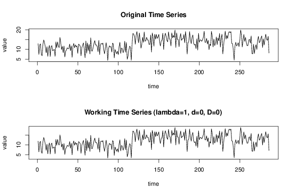
plot(ox,type='l',main='Original Time Series',xlab='time',ylab='value')
if (par8=='') {
mytitle <- paste('Working Time Series (lambda=',par2,', d=',par3,', D=',par4,')',sep='')
mysub <- paste('(lambda=',par2,', d=',par3,', D=',par4,', CI=', par7, ', CI type=',par6,')',sep='')
} else {
mytitle <- paste('Working Time Series (base=',par8,', d=',par3,', D=',par4,')',sep='')
mysub <- paste('(base=',par8,', d=',par3,', D=',par4,', CI=', par7, ', CI type=',par6,')',sep='')
}
plot(x,type='l', main=mytitle,xlab='time',ylab='value')
par(op)
dev.off()
bitmap(file='pic1.png')
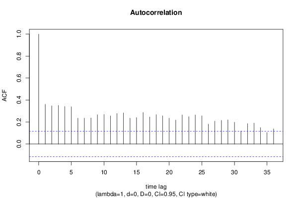
racf <- acf(x, par1, main='Autocorrelation', xlab='time lag', ylab='ACF', ci.type=par6, ci=par7, sub=mysub)
dev.off()
bitmap(file='pic2.png')
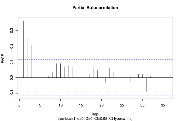
rpacf <- pacf(x,par1,main='Partial Autocorrelation',xlab='lags',ylab='PACF',sub=mysub)
dev.off()
(myacf <- c(racf$acf))
(mypacf <- c(rpacf$acf))
lengthx <- length(x)
sqrtn <- sqrt(lengthx)
load(file='createtable')
a<-table.start()
a<-table.row.start(a)
a<-table.element(a,'Autocorrelation Function',4,TRUE)
a<-table.row.end(a)
a<-table.row.start(a)
a<-table.element(a,'Time lag k',header=TRUE)
a<-table.element(a,hyperlink('basics.htm','ACF(k)','click here for more information about the Autocorrelation Function'),header=TRUE)
a<-table.element(a,'T-STAT',header=TRUE)
a<-table.element(a,'P-value',header=TRUE)
a<-table.row.end(a)
for (i in 2:(par1+1)) {
a<-table.row.start(a)
a<-table.element(a,i-1,header=TRUE)
a<-table.element(a,round(myacf[i],6))
mytstat <- myacf[i]*sqrtn
a<-table.element(a,round(mytstat,4))
a<-table.element(a,round(1-pt(abs(mytstat),lengthx),6))
a<-table.row.end(a)
}
a<-table.end(a)
table.save(a,file='mytable.tab')
a<-table.start()
a<-table.row.start(a)
a<-table.element(a,'Partial Autocorrelation Function',4,TRUE)
a<-table.row.end(a)
a<-table.row.start(a)
a<-table.element(a,'Time lag k',header=TRUE)
a<-table.element(a,hyperlink('basics.htm','PACF(k)','click here for more information about the Partial Autocorrelation Function'),header=TRUE)
a<-table.element(a,'T-STAT',header=TRUE)
a<-table.element(a,'P-value',header=TRUE)
a<-table.row.end(a)
for (i in 1:par1) {
a<-table.row.start(a)
a<-table.element(a,i,header=TRUE)
a<-table.element(a,round(mypacf[i],6))
mytstat <- mypacf[i]*sqrtn
a<-table.element(a,round(mytstat,4))
a<-table.element(a,round(1-pt(abs(mytstat),lengthx),6))
a<-table.row.end(a)
}
a<-table.end(a)
table.save(a,file='mytable1.tab')

Free Statistics

Description of Statistical Computation

Tree of Dependent Computations

Dataset

Tables (Output of Computation)

Figures (Output of Computation)

Input Parameters & R Code