Repository of Reproducible Computations

Free Statistics

of Irreproducible Research!

Author's title

Author

*The author of this computation has been verified*

R Software Module

rwasp_Two Factor ANOVA.wasp

Title produced by software

Two-Way ANOVA

Date of computation

Wed, 17 Dec 2014 19:25:56 +0000

Cite this page as follows

Statistical Computations at FreeStatistics.org, Office for Research Development and Education, URL https://freestatistics.org/blog/index.php?v=date/2014/Dec/17/t1418844556xt0d37vu0tbehdp.htm/, Retrieved Thu, 16 May 2024 12:59:20 +0000

Statistical Computations at FreeStatistics.org, Office for Research Development and Education, URL https://freestatistics.org/blog/index.php?pk=270599, Retrieved Thu, 16 May 2024 12:59:20 +0000

QR Codes:

Paste this QR Code to cite your computation.

Original text written by user:

IsPrivate?

No (this computation is public)

User-defined keywords

Estimated Impact

Family? (F = Feedback message, R = changed R code, M = changed R Module, P = changed Parameters, D = changed Data)

-       [Two-Way ANOVA] [] [2014-12-17 19:25:56] [18673d63f90870b9c004059cd6229007] [Current]

Feedback Forum

Post a new message

Dataseries X:

Download CSV

Histogram

Boxplots

'S' 1 7.5
'S' 0 6
'S' 1 6.5
'S' 0 1
'S' 1 1
'S' 1 5.5
'S' 1 8.5
'S' 0 6.5
'S' 1 4.5
'S' 1 2
'S' 1 5
'S' 1 0.5
'S' 1 5
'S' 1 5
'S' 0 2.5
'B' 0 5
'S' 0 5.5
'S' 1 3.5
'B' 0 3
'S' 1 4
'S' 0 0.5
'S' 1 6.5
'S' 1 4.5
'S' 0 7.5
'S' 1 5.5
'S' 1 4
'B' 1 7.5
'B' 1 7
'S' 0 4
'S' 1 5.5
'S' 0 2.5
'S' 0 5.5
'S' 1 3.5
'S' 1 2.5
'S' 1 4.5
'S' 1 4.5
'S' 1 4.5
'B' 0 6
'S' 1 2.5
'S' 1 5
'S' 0 0
'S' 1 5
'S' 1 6.5
'S' 1 5
'B' 1 6
'S' 1 4.5
'S' 0 5.5
'B' 1 1
'S' 1 7.5
'B' 0 6
'B' 1 5
'B' 1 1
'S' 1 5
'B' 1 6.5
'S' 1 7
'S' 1 4.5
'B' 1 0
'S' 0 8.5
'B' 1 3.5
'B' 0 7.5
'S' 1 3.5
'S' 1 6
'S' 0 1.5
'S' 0 9
'S' 1 3.5
'B' 0 3.5
'S' 1 4
'S' 0 6.5
'S' 1 7.5
'B' 1 6
'S' 0 5
'S' 0 5.5
'B' 0 3.5
'B' 0 7.5
'S' 1 6.5
'S' 1 6.5
'B' 0 6.5
'S' 1 7
'B' 0 3.5
'S' 0 1.5
'B' 1 4
'B' 0 7.5
'B' 0 4.5
'B' 0 0
'B' 1 3.5
'B' 0 5.5
'B' 1 5
'B' 1 4.5
'B' 0 2.5
'B' 0 7.5
'B' 0 7
'B' 1 0
'B' 1 4.5
'B' 1 3
'B' 0 1.5
'B' 1 3.5
'B' 0 2.5
'B' 1 5.5
'B' 1 8
'B' 1 1
'B' 1 5
'B' 1 4.5
'B' 0 3
'B' 1 3
'B' 1 8
'B' 1 2.5
'B' 0 7
'B' 0 0
'B' 0 1
'B' 0 3.5
'B' 0 5.5
'B' 0 5.5
'S' 1 0.5
'S' 1 7.5
'S' 1 9
'S' 1 9.5
'B' 1 8.5
'B' 0 7
'S' 1 8
'S' 1 10
'S' 0 7
'S' 1 8.5
'S' 0 9
'S' 0 9.5
'S' 1 4
'S' 1 6
'S' 1 8
'S' 1 5.5
'B' 1 9.5
'S' 1 7.5
'S' 1 7
'S' 1 7.5
'S' 0 8
'S' 1 7
'S' 1 7
'S' 1 6
'S' 1 10
'S' 1 2.5
'S' 1 9
'S' 0 8
'B' 1 6
'S' 1 8.5
'S' 1 6
'S' 1 9
'S' 0 8
'S' 0 9
'S' 0 5.5
'S' 0 7
'S' 0 5.5
'S' 0 9
'S' 1 2
'S' 0 8.5
'S' 1 9
'S' 1 8.5
'B' 0 9
'B' 1 7.5
'S' 1 10
'S' 1 9
'B' 0 7.5
'B' 0 6
'B' 0 10.5
'B' 0 8.5
'S' 1 8
'S' 0 10
'B' 1 10.5
'B' 0 6.5
'B' 1 9.5
'B' 0 8.5
'B' 1 7.5
'B' 0 5
'B' 0 8
'B' 1 10
'B' 0 7
'S' 1 7.5
'S' 1 7.5
'B' 1 9.5
'S' 1 6
'S' 1 10
'B' 0 7
'S' 1 3
'B' 0 6
'B' 0 7
'S' 0 10
'B' 1 7
'B' 0 3.5
'B' 1 8
'B' 0 10
'B' 0 5.5
'B' 0 6
'B' 0 6.5
'B' 1 6.5
'B' 1 8.5
'B' 1 4
'B' 1 9.5
'B' 0 8
'B' 0 8.5
'S' 1 5.5
'B' 0 7
'B' 0 9
'B' 0 8
'S' 0 10
'B' 1 8
'S' 1 6
'B' 0 8
'S' 0 5
'B' 1 9
'S' 0 4.5
'B' 1 8.5
'B' 1 9.5
'B' 0 8.5
'B' 1 7.5
'S' 1 7.5
'S' 1 5
'B' 0 7
'S' 0 8
'S' 0 5.5
'B' 1 8.5
'S' 0 9.5
'B' 1 7
'B' 1 8
'S' 0 8.5
'B' 0 3.5
'S' 0 6.5
'S' 1 6.5
'S' 1 10.5
'B' 0 8.5
'S' 0 8
'B' 0 10
'S' 1 10
'S' 1 9.5
'S' 0 9
'S' 0 10
'B' 0 7.5
'S' 1 4.5
'S' 1 4.5
'S' 1 0.5
'B' 1 6.5
'S' 0 4.5
'S' 1 5.5
'B' 1 5
'S' 1 6
'B' 0 4
'B' 0 8
'B' 1 10.5
'B' 1 6.5
'B' 1 8
'S' 1 8.5
'S' 0 5.5
'S' 1 7
'S' 0 5
'S' 1 3.5
'S' 1 5
'B' 0 9
'B' 1 8.5
'S' 0 5
'B' 1 9.5
'B' 0 3
'S' 1 1.5
'B' 0 6
'B' 0 0.5
'B' 1 6.5
'B' 1 7.5
'B' 0 4.5
'B' 1 8
'B' 1 9
'B' 0 7.5
'B' 1 8.5
'B' 0 7
'B' 0 9.5
'B' 1 6.5
'B' 1 9.5
'B' 0 6
'B' 1 8
'B' 0 9.5
'B' 0 8
'S' 1 8
'B' 0 9
'B' 0 5

Summary of computational transaction
Raw Input	view raw input (R code)
Raw Output	view raw output of R engine
Computing time	3 seconds
R Server	'Gertrude Mary Cox' @ cox.wessa.net

\begin{tabular}{lllllllll}
\hline
Summary of computational transaction \tabularnewline
Raw Input & view raw input (R code)  \tabularnewline
Raw Output & view raw output of R engine  \tabularnewline
Computing time & 3 seconds \tabularnewline
R Server & 'Gertrude Mary Cox' @ cox.wessa.net \tabularnewline
\hline
\end{tabular}
%Source: https://freestatistics.org/blog/index.php?pk=270599&T=0

[TABLE]
[ROW][C]Summary of computational transaction[/C][/ROW]
[ROW][C]Raw Input[/C][C]view raw input (R code) [/C][/ROW]
[ROW][C]Raw Output[/C][C]view raw output of R engine [/C][/ROW]
[ROW][C]Computing time[/C][C]3 seconds[/C][/ROW]
[ROW][C]R Server[/C][C]'Gertrude Mary Cox' @ cox.wessa.net[/C][/ROW]
[/TABLE]
Source: https://freestatistics.org/blog/index.php?pk=270599&T=0

Globally Unique Identifier (entire table): ba.freestatistics.org/blog/index.php?pk=270599&T=0

As an alternative you can also use a QR Code:

The GUIDs for individual cells are displayed in the table below:

Summary of computational transaction
Raw Input	view raw input (R code)
Raw Output	view raw output of R engine
Computing time	3 seconds
R Server	'Gertrude Mary Cox' @ cox.wessa.net

ANOVA Model
Response ~ Treatment_A * Treatment_B
means	6.125	0.187	0.359	-0.714

\begin{tabular}{lllllllll}
\hline
ANOVA Model \tabularnewline
Response ~ Treatment_A * Treatment_B \tabularnewline
means & 6.125 & 0.187 & 0.359 & -0.714 \tabularnewline
\hline
\end{tabular}
%Source: https://freestatistics.org/blog/index.php?pk=270599&T=1

[TABLE]
[ROW][C]ANOVA Model[/C][/ROW]
[ROW][C]Response ~ Treatment_A * Treatment_B[/C][/ROW]
[ROW][C]means[/C][C]6.125[/C][C]0.187[/C][C]0.359[/C][C]-0.714[/C][/ROW]
[/TABLE]
Source: https://freestatistics.org/blog/index.php?pk=270599&T=1

Globally Unique Identifier (entire table): ba.freestatistics.org/blog/index.php?pk=270599&T=1

As an alternative you can also use a QR Code:

The GUIDs for individual cells are displayed in the table below:

ANOVA Model
Response ~ Treatment_A * Treatment_B
means	6.125	0.187	0.359	-0.714

ANOVA Statistics
	Df	Sum Sq	Mean Sq	F value	Pr(>F)
	1
Treatment_A	1	3.261	3.261	0.506	0.478
Treatment_B	1	0.012	0.012	0.002	0.965
Treatment_A:Treatment_B	1	8.369	8.369	1.298	0.256
Residuals	274	1766.502	6.447

\begin{tabular}{lllllllll}
\hline
ANOVA Statistics \tabularnewline
  & Df & Sum Sq & Mean Sq & F value & Pr(>F) \tabularnewline
 & 1 &  &  &  &  \tabularnewline
Treatment_A & 1 & 3.261 & 3.261 & 0.506 & 0.478 \tabularnewline
Treatment_B & 1 & 0.012 & 0.012 & 0.002 & 0.965 \tabularnewline
Treatment_A:Treatment_B & 1 & 8.369 & 8.369 & 1.298 & 0.256 \tabularnewline
Residuals & 274 & 1766.502 & 6.447 &   &   \tabularnewline
\hline
\end{tabular}
%Source: https://freestatistics.org/blog/index.php?pk=270599&T=2

[TABLE]
[ROW][C]ANOVA Statistics[/C][/ROW]
[ROW][C] [/C][C]Df[/C][C]Sum Sq[/C][C]Mean Sq[/C][C]F value[/C][C]Pr(>F)[/C][/ROW]
[ROW][C][/C][C]1[/C][C][/C][C][/C][C][/C][C][/C][/ROW]
[ROW][C]Treatment_A[/C][C]1[/C][C]3.261[/C][C]3.261[/C][C]0.506[/C][C]0.478[/C][/ROW]
[ROW][C]Treatment_B[/C][C]1[/C][C]0.012[/C][C]0.012[/C][C]0.002[/C][C]0.965[/C][/ROW]
[ROW][C]Treatment_A:Treatment_B[/C][C]1[/C][C]8.369[/C][C]8.369[/C][C]1.298[/C][C]0.256[/C][/ROW]
[ROW][C]Residuals[/C][C]274[/C][C]1766.502[/C][C]6.447[/C][C] [/C][C] [/C][/ROW]
[/TABLE]
Source: https://freestatistics.org/blog/index.php?pk=270599&T=2

Globally Unique Identifier (entire table): ba.freestatistics.org/blog/index.php?pk=270599&T=2

As an alternative you can also use a QR Code:

The GUIDs for individual cells are displayed in the table below:

ANOVA Statistics
	Df	Sum Sq	Mean Sq	F value	Pr(>F)
	1
Treatment_A	1	3.261	3.261	0.506	0.478
Treatment_B	1	0.012	0.012	0.002	0.965
Treatment_A:Treatment_B	1	8.369	8.369	1.298	0.256
Residuals	274	1766.502	6.447

Tukey Honest Significant Difference Comparisons
	diff	lwr	upr	p adj
S-B	-0.217	-0.816	0.383	0.478
1-0	0.013	-0.592	0.618	0.966
S:0-B:0	0.187	-1.035	1.41	0.979
B:1-B:0	0.359	-0.768	1.487	0.843
S:1-B:0	-0.168	-1.195	0.86	0.975
B:1-S:0	0.172	-1.081	1.425	0.985
S:1-S:0	-0.355	-1.519	0.809	0.86
S:1-B:1	-0.527	-1.591	0.537	0.576

\begin{tabular}{lllllllll}
\hline
Tukey Honest Significant Difference Comparisons \tabularnewline
  & diff & lwr & upr & p adj \tabularnewline
S-B & -0.217 & -0.816 & 0.383 & 0.478 \tabularnewline
1-0 & 0.013 & -0.592 & 0.618 & 0.966 \tabularnewline
S:0-B:0 & 0.187 & -1.035 & 1.41 & 0.979 \tabularnewline
B:1-B:0 & 0.359 & -0.768 & 1.487 & 0.843 \tabularnewline
S:1-B:0 & -0.168 & -1.195 & 0.86 & 0.975 \tabularnewline
B:1-S:0 & 0.172 & -1.081 & 1.425 & 0.985 \tabularnewline
S:1-S:0 & -0.355 & -1.519 & 0.809 & 0.86 \tabularnewline
S:1-B:1 & -0.527 & -1.591 & 0.537 & 0.576 \tabularnewline
\hline
\end{tabular}
%Source: https://freestatistics.org/blog/index.php?pk=270599&T=3

[TABLE]
[ROW][C]Tukey Honest Significant Difference Comparisons[/C][/ROW]
[ROW][C] [/C][C]diff[/C][C]lwr[/C][C]upr[/C][C]p adj[/C][/ROW]
[ROW][C]S-B[/C][C]-0.217[/C][C]-0.816[/C][C]0.383[/C][C]0.478[/C][/ROW]
[ROW][C]1-0[/C][C]0.013[/C][C]-0.592[/C][C]0.618[/C][C]0.966[/C][/ROW]
[ROW][C]S:0-B:0[/C][C]0.187[/C][C]-1.035[/C][C]1.41[/C][C]0.979[/C][/ROW]
[ROW][C]B:1-B:0[/C][C]0.359[/C][C]-0.768[/C][C]1.487[/C][C]0.843[/C][/ROW]
[ROW][C]S:1-B:0[/C][C]-0.168[/C][C]-1.195[/C][C]0.86[/C][C]0.975[/C][/ROW]
[ROW][C]B:1-S:0[/C][C]0.172[/C][C]-1.081[/C][C]1.425[/C][C]0.985[/C][/ROW]
[ROW][C]S:1-S:0[/C][C]-0.355[/C][C]-1.519[/C][C]0.809[/C][C]0.86[/C][/ROW]
[ROW][C]S:1-B:1[/C][C]-0.527[/C][C]-1.591[/C][C]0.537[/C][C]0.576[/C][/ROW]
[/TABLE]
Source: https://freestatistics.org/blog/index.php?pk=270599&T=3

Globally Unique Identifier (entire table): ba.freestatistics.org/blog/index.php?pk=270599&T=3

As an alternative you can also use a QR Code:

The GUIDs for individual cells are displayed in the table below:

Tukey Honest Significant Difference Comparisons
	diff	lwr	upr	p adj
S-B	-0.217	-0.816	0.383	0.478
1-0	0.013	-0.592	0.618	0.966
S:0-B:0	0.187	-1.035	1.41	0.979
B:1-B:0	0.359	-0.768	1.487	0.843
S:1-B:0	-0.168	-1.195	0.86	0.975
B:1-S:0	0.172	-1.081	1.425	0.985
S:1-S:0	-0.355	-1.519	0.809	0.86
S:1-B:1	-0.527	-1.591	0.537	0.576

Levenes Test for Homogeneity of Variance
	Df	F value	Pr(>F)
Group	3	0.342	0.795
	274

\begin{tabular}{lllllllll}
\hline
Levenes Test for Homogeneity of Variance \tabularnewline
  & Df & F value & Pr(>F) \tabularnewline
Group & 3 & 0.342 & 0.795 \tabularnewline
  & 274 &   &   \tabularnewline
\hline
\end{tabular}
%Source: https://freestatistics.org/blog/index.php?pk=270599&T=4

[TABLE]
[ROW][C]Levenes Test for Homogeneity of Variance[/C][/ROW]
[ROW][C] [/C][C]Df[/C][C]F value[/C][C]Pr(>F)[/C][/ROW]
[ROW][C]Group[/C][C]3[/C][C]0.342[/C][C]0.795[/C][/ROW]
[ROW][C] [/C][C]274[/C][C] [/C][C] [/C][/ROW]
[/TABLE]
Source: https://freestatistics.org/blog/index.php?pk=270599&T=4

Globally Unique Identifier (entire table): ba.freestatistics.org/blog/index.php?pk=270599&T=4

As an alternative you can also use a QR Code:

The GUIDs for individual cells are displayed in the table below:

Levenes Test for Homogeneity of Variance
	Df	F value	Pr(>F)
Group	3	0.342	0.795
	274

Figure 1

PNG link

Postscript link

PDF link

Figure 2

PNG link

Postscript link

PDF link

Figure 3

PNG link

Postscript link

PDF link

Figure 4

PNG link

Postscript link

PDF link

Parameters (Session):

par1 = 3 ; par2 = 1 ; par3 = 2 ; par4 = TRUE ;

Parameters (R input):

par1 = 3 ; par2 = 1 ; par3 = 2 ; par4 = TRUE ;

R code (references can be found in the software module):

cat1 <- as.numeric(par1) #
cat2<- as.numeric(par2) #
cat3 <- as.numeric(par3)
intercept<-as.logical(par4)
x <- t(x)
x1<-as.numeric(x[,cat1])
f1<-as.character(x[,cat2])
f2 <- as.character(x[,cat3])
xdf<-data.frame(x1,f1, f2)
(V1<-dimnames(y)[[1]][cat1])
(V2<-dimnames(y)[[1]][cat2])
(V3 <-dimnames(y)[[1]][cat3])
names(xdf)<-c('Response', 'Treatment_A', 'Treatment_B')
if(intercept == FALSE) (lmxdf<-lm(Response ~ Treatment_A * Treatment_B- 1, data = xdf) ) else (lmxdf<-lm(Response ~ Treatment_A * Treatment_B, data = xdf) )
(aov.xdf<-aov(lmxdf) )
(anova.xdf<-anova(lmxdf) )
load(file='createtable')
a<-table.start()
a<-table.row.start(a)
a<-table.element(a,'ANOVA Model', length(lmxdf$coefficients)+1,TRUE)
a<-table.row.end(a)
a<-table.row.start(a)
a<-table.element(a, lmxdf$call['formula'],length(lmxdf$coefficients)+1,TRUE)
a<-table.row.end(a)
a<-table.row.start(a)
a<-table.element(a, 'means',,TRUE)
for(i in 1:length(lmxdf$coefficients)){
a<-table.element(a, round(lmxdf$coefficients[i], digits=3),,FALSE)
}
a<-table.row.end(a)
a<-table.end(a)
table.save(a,file='mytable.tab')
a<-table.start()
a<-table.row.start(a)
a<-table.element(a,'ANOVA Statistics', 5+1,TRUE)
a<-table.row.end(a)
a<-table.row.start(a)
a<-table.element(a, ' ',,TRUE)
a<-table.element(a, 'Df',,FALSE)
a<-table.element(a, 'Sum Sq',,FALSE)
a<-table.element(a, 'Mean Sq',,FALSE)
a<-table.element(a, 'F value',,FALSE)
a<-table.element(a, 'Pr(>F)',,FALSE)
a<-table.row.end(a)
for(i in 1 : length(rownames(anova.xdf))-1){
a<-table.row.start(a)
a<-table.element(a,rownames(anova.xdf)[i] ,,TRUE)
a<-table.element(a, anova.xdf$Df[1],,FALSE)
a<-table.element(a, round(anova.xdf$'Sum Sq'[i], digits=3),,FALSE)
a<-table.element(a, round(anova.xdf$'Mean Sq'[i], digits=3),,FALSE)
a<-table.element(a, round(anova.xdf$'F value'[i], digits=3),,FALSE)
a<-table.element(a, round(anova.xdf$'Pr(>F)'[i], digits=3),,FALSE)
a<-table.row.end(a)
}
a<-table.row.start(a)
a<-table.element(a, 'Residuals',,TRUE)
a<-table.element(a, anova.xdf$'Df'[i+1],,FALSE)
a<-table.element(a, round(anova.xdf$'Sum Sq'[i+1], digits=3),,FALSE)
a<-table.element(a, round(anova.xdf$'Mean Sq'[i+1], digits=3),,FALSE)
a<-table.element(a, ' ',,FALSE)
a<-table.element(a, ' ',,FALSE)
a<-table.row.end(a)
a<-table.end(a)
table.save(a,file='mytable1.tab')
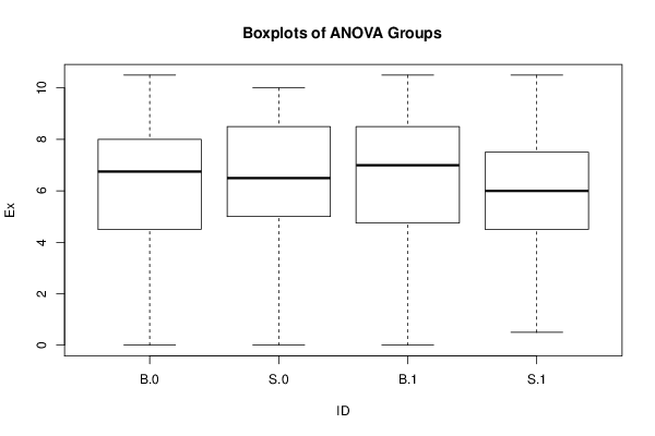
bitmap(file='anovaplot.png')
boxplot(Response ~ Treatment_A + Treatment_B, data=xdf, xlab=V2, ylab=V1, main='Boxplots of ANOVA Groups')
dev.off()
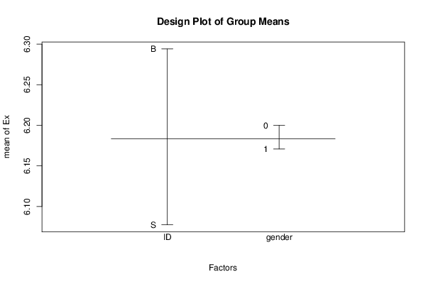
bitmap(file='designplot.png')
xdf2 <- xdf # to preserve xdf make copy for function
names(xdf2) <- c(V1, V2, V3)
plot.design(xdf2, main='Design Plot of Group Means')
dev.off()
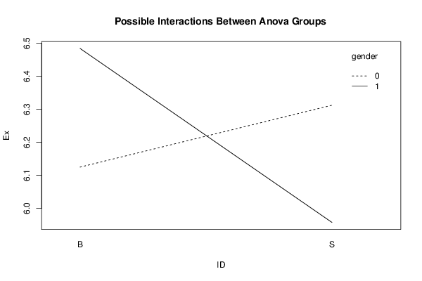
bitmap(file='interactionplot.png')
interaction.plot(xdf$Treatment_A, xdf$Treatment_B, xdf$Response, xlab=V2, ylab=V1, trace.label=V3, main='Possible Interactions Between Anova Groups')
dev.off()
if(intercept==TRUE){
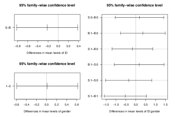
thsd<-TukeyHSD(aov.xdf)
names(thsd) <- c(V2, V3, paste(V2, ':', V3, sep=''))
bitmap(file='TukeyHSDPlot.png')
layout(matrix(c(1,2,3,3), 2,2))
plot(thsd, las=1)
dev.off()
}
if(intercept==TRUE){
ntables<-length(names(thsd))
a<-table.start()
a<-table.row.start(a)
a<-table.element(a,'Tukey Honest Significant Difference Comparisons', 5,TRUE)
a<-table.row.end(a)
a<-table.row.start(a)
a<-table.element(a, ' ', 1, TRUE)
for(i in 1:4){
a<-table.element(a,colnames(thsd[[1]])[i], 1, TRUE)
}
a<-table.row.end(a)
for(nt in 1:ntables){
for(i in 1:length(rownames(thsd[[nt]]))){
a<-table.row.start(a)
a<-table.element(a,rownames(thsd[[nt]])[i], 1, TRUE)
for(j in 1:4){
a<-table.element(a,round(thsd[[nt]][i,j], digits=3), 1, FALSE)
}
a<-table.row.end(a)
}
} # end nt
a<-table.end(a)
table.save(a,file='hsdtable.tab')
}#end if hsd tables
if(intercept==FALSE){
a<-table.start()
a<-table.row.start(a)
a<-table.element(a,'TukeyHSD Message', 1,TRUE)
a<-table.row.end(a)
a<-table.start()
a<-table.row.start(a)
a<-table.element(a,'Must Include Intercept to use Tukey Test ', 1, FALSE)
a<-table.row.end(a)
a<-table.end(a)
table.save(a,file='mytable2.tab')
}
library(car)
lt.lmxdf<-levene.test(lmxdf)
a<-table.start()
a<-table.row.start(a)
a<-table.element(a,'Levenes Test for Homogeneity of Variance', 4,TRUE)
a<-table.row.end(a)
a<-table.row.start(a)
a<-table.element(a,' ', 1, TRUE)
for (i in 1:3){
a<-table.element(a,names(lt.lmxdf)[i], 1, FALSE)
}
a<-table.row.end(a)
a<-table.row.start(a)
a<-table.element(a,'Group', 1, TRUE)
for (i in 1:3){
a<-table.element(a,round(lt.lmxdf[[i]][1], digits=3), 1, FALSE)
}
a<-table.row.end(a)
a<-table.row.start(a)
a<-table.element(a,' ', 1, TRUE)
a<-table.element(a,lt.lmxdf[[1]][2], 1, FALSE)
a<-table.element(a,' ', 1, FALSE)
a<-table.element(a,' ', 1, FALSE)
a<-table.row.end(a)
a<-table.end(a)
table.save(a,file='mytable3.tab')

Free Statistics

Description of Statistical Computation

Tree of Dependent Computations

Dataset

Tables (Output of Computation)

Figures (Output of Computation)

Input Parameters & R Code