Free Statistics
of Irreproducible Research!
Description of Statistical Computation | |||||||||||||||||||||||||||||||||||||||||||||||||||||||||||||||||||||||||||||||||||||||||||||||||||||||||||||
|---|---|---|---|---|---|---|---|---|---|---|---|---|---|---|---|---|---|---|---|---|---|---|---|---|---|---|---|---|---|---|---|---|---|---|---|---|---|---|---|---|---|---|---|---|---|---|---|---|---|---|---|---|---|---|---|---|---|---|---|---|---|---|---|---|---|---|---|---|---|---|---|---|---|---|---|---|---|---|---|---|---|---|---|---|---|---|---|---|---|---|---|---|---|---|---|---|---|---|---|---|---|---|---|---|---|---|---|---|---|
| Author's title | |||||||||||||||||||||||||||||||||||||||||||||||||||||||||||||||||||||||||||||||||||||||||||||||||||||||||||||
| Author | *The author of this computation has been verified* | ||||||||||||||||||||||||||||||||||||||||||||||||||||||||||||||||||||||||||||||||||||||||||||||||||||||||||||
| R Software Module | rwasp_correlation.wasp | ||||||||||||||||||||||||||||||||||||||||||||||||||||||||||||||||||||||||||||||||||||||||||||||||||||||||||||
| Title produced by software | Pearson Correlation | ||||||||||||||||||||||||||||||||||||||||||||||||||||||||||||||||||||||||||||||||||||||||||||||||||||||||||||
| Date of computation | Thu, 18 Dec 2014 07:42:53 +0000 | ||||||||||||||||||||||||||||||||||||||||||||||||||||||||||||||||||||||||||||||||||||||||||||||||||||||||||||
| Cite this page as follows | Statistical Computations at FreeStatistics.org, Office for Research Development and Education, URL https://freestatistics.org/blog/index.php?v=date/2014/Dec/18/t14188885974n7f3u8wbgwf9zq.htm/, Retrieved Fri, 17 May 2024 13:57:00 +0000 | ||||||||||||||||||||||||||||||||||||||||||||||||||||||||||||||||||||||||||||||||||||||||||||||||||||||||||||
| Statistical Computations at FreeStatistics.org, Office for Research Development and Education, URL https://freestatistics.org/blog/index.php?pk=270752, Retrieved Fri, 17 May 2024 13:57:00 +0000 | |||||||||||||||||||||||||||||||||||||||||||||||||||||||||||||||||||||||||||||||||||||||||||||||||||||||||||||
| QR Codes: | |||||||||||||||||||||||||||||||||||||||||||||||||||||||||||||||||||||||||||||||||||||||||||||||||||||||||||||
|
| |||||||||||||||||||||||||||||||||||||||||||||||||||||||||||||||||||||||||||||||||||||||||||||||||||||||||||||
| Original text written by user: | |||||||||||||||||||||||||||||||||||||||||||||||||||||||||||||||||||||||||||||||||||||||||||||||||||||||||||||
| IsPrivate? | No (this computation is public) | ||||||||||||||||||||||||||||||||||||||||||||||||||||||||||||||||||||||||||||||||||||||||||||||||||||||||||||
| User-defined keywords | |||||||||||||||||||||||||||||||||||||||||||||||||||||||||||||||||||||||||||||||||||||||||||||||||||||||||||||
| Estimated Impact | 130 | ||||||||||||||||||||||||||||||||||||||||||||||||||||||||||||||||||||||||||||||||||||||||||||||||||||||||||||
Tree of Dependent Computations | |||||||||||||||||||||||||||||||||||||||||||||||||||||||||||||||||||||||||||||||||||||||||||||||||||||||||||||
| Family? (F = Feedback message, R = changed R code, M = changed R Module, P = changed Parameters, D = changed Data) | |||||||||||||||||||||||||||||||||||||||||||||||||||||||||||||||||||||||||||||||||||||||||||||||||||||||||||||
| - [Percentiles] [Intrinsic Motivat...] [2010-10-12 12:10:58] [b98453cac15ba1066b407e146608df68] - RMPD [Kernel Density Estimation] [] [2011-10-18 22:42:23] [b98453cac15ba1066b407e146608df68] - RMPD [Percentiles] [] [2011-10-18 22:46:45] [b98453cac15ba1066b407e146608df68] - RMPD [Notched Boxplots] [] [2011-10-18 22:58:56] [b98453cac15ba1066b407e146608df68] - RMP [Notched Boxplots] [] [2014-10-16 18:35:18] [bcf5edf18529a33bd1494456d2c6cb9a] - RMPD [Pearson Correlation] [] [2014-12-18 07:42:53] [88f8137dd67cdcd531568536dca46410] [Current] | |||||||||||||||||||||||||||||||||||||||||||||||||||||||||||||||||||||||||||||||||||||||||||||||||||||||||||||
| Feedback Forum | |||||||||||||||||||||||||||||||||||||||||||||||||||||||||||||||||||||||||||||||||||||||||||||||||||||||||||||
Post a new message | |||||||||||||||||||||||||||||||||||||||||||||||||||||||||||||||||||||||||||||||||||||||||||||||||||||||||||||
Dataset | |||||||||||||||||||||||||||||||||||||||||||||||||||||||||||||||||||||||||||||||||||||||||||||||||||||||||||||
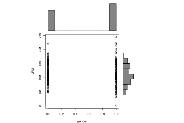
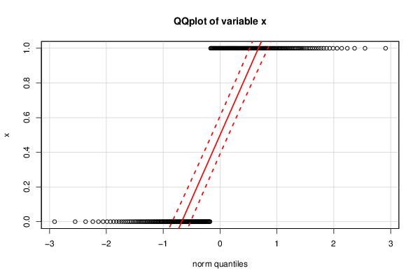
| Dataseries X: | |||||||||||||||||||||||||||||||||||||||||||||||||||||||||||||||||||||||||||||||||||||||||||||||||||||||||||||
0 1 0 1 1 1 0 1 1 1 1 1 1 0 0 0 1 0 1 0 1 1 0 1 1 1 1 0 1 0 0 0 1 1 1 1 0 1 1 0 1 1 1 1 1 0 1 1 0 1 1 1 1 1 1 1 0 1 0 1 1 0 0 1 0 1 0 1 1 0 0 0 0 1 0 0 1 0 0 1 0 0 0 1 0 1 1 0 0 0 1 1 1 0 1 0 1 1 1 1 1 0 1 1 1 0 0 0 0 0 0 1 1 1 1 1 0 1 1 0 1 0 0 1 1 1 1 1 1 1 1 0 1 1 1 1 1 1 0 1 1 1 1 1 0 0 1 0 0 1 0 1 1 0 1 1 1 0 0 0 0 1 0 1 0 1 0 1 0 0 1 0 1 1 1 1 1 0 1 0 0 0 1 0 1 0 0 0 0 1 1 1 1 0 0 1 0 0 0 0 1 1 0 0 1 0 1 1 0 1 1 1 0 0 0 1 1 1 1 0 0 0 1 1 0 0 0 1 1 0 0 0 1 1 1 1 0 1 1 1 0 0 1 0 1 1 0 1 0 1 1 0 1 0 1 0 1 0 0 1 1 0 1 1 0 1 0 0 1 1 0 1 0 0 1 0 0 1 | |||||||||||||||||||||||||||||||||||||||||||||||||||||||||||||||||||||||||||||||||||||||||||||||||||||||||||||
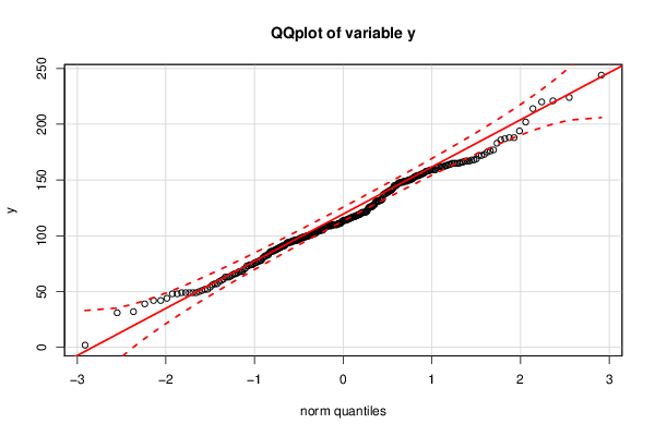
| Dataseries Y: | |||||||||||||||||||||||||||||||||||||||||||||||||||||||||||||||||||||||||||||||||||||||||||||||||||||||||||||
91 137 92 148 131 59 128 90 83 116 42 155 96 49 104 76 66 74 99 96 108 97 116 106 80 74 114 87 140 127 74 91 98 126 98 95 133 110 70 95 86 130 96 99 68 121 131 71 102 68 89 87 49 96 100 141 102 110 100 146 147 94 52 61 98 60 118 109 68 109 115 78 118 73 162 122 65 100 82 52 115 90 121 101 104 42 96 110 108 113 57 86 88 115 85 111 102 86 114 94 64 77 105 49 95 89 78 110 117 63 131 102 63 117 57 73 77 105 31 112 139 49 56 158 128 224 105 159 167 165 159 48 119 163 153 148 188 149 63 244 150 132 161 105 162 81 97 110 104 166 88 111 145 99 162 163 109 76 109 120 91 148 108 125 119 116 149 138 148 159 164 176 202 214 188 110 48 54 50 124 121 221 150 153 154 94 156 151 157 194 159 39 100 187 105 111 162 99 186 183 138 101 177 126 101 139 114 114 162 111 75 82 159 158 67 121 32 117 165 147 165 150 154 126 149 145 109 120 172 132 169 172 114 156 167 2 113 165 165 118 173 158 155 49 220 122 151 44 141 152 103 107 175 154 110 143 131 167 137 121 168 149 94 51 168 145 140 109 66 119 164 132 126 83 142 93 117 166 | |||||||||||||||||||||||||||||||||||||||||||||||||||||||||||||||||||||||||||||||||||||||||||||||||||||||||||||
Tables (Output of Computation) | |||||||||||||||||||||||||||||||||||||||||||||||||||||||||||||||||||||||||||||||||||||||||||||||||||||||||||||
| |||||||||||||||||||||||||||||||||||||||||||||||||||||||||||||||||||||||||||||||||||||||||||||||||||||||||||||
Figures (Output of Computation) | |||||||||||||||||||||||||||||||||||||||||||||||||||||||||||||||||||||||||||||||||||||||||||||||||||||||||||||
Input Parameters & R Code | |||||||||||||||||||||||||||||||||||||||||||||||||||||||||||||||||||||||||||||||||||||||||||||||||||||||||||||
| Parameters (Session): | |||||||||||||||||||||||||||||||||||||||||||||||||||||||||||||||||||||||||||||||||||||||||||||||||||||||||||||
| Parameters (R input): | |||||||||||||||||||||||||||||||||||||||||||||||||||||||||||||||||||||||||||||||||||||||||||||||||||||||||||||
| R code (references can be found in the software module): | |||||||||||||||||||||||||||||||||||||||||||||||||||||||||||||||||||||||||||||||||||||||||||||||||||||||||||||
x <- x[!is.na(y)] | |||||||||||||||||||||||||||||||||||||||||||||||||||||||||||||||||||||||||||||||||||||||||||||||||||||||||||||