Free Statistics
of Irreproducible Research!
Description of Statistical Computation | |||||||||||||||||||||||||||||||||||||||||||||||||||||||||||||||||
|---|---|---|---|---|---|---|---|---|---|---|---|---|---|---|---|---|---|---|---|---|---|---|---|---|---|---|---|---|---|---|---|---|---|---|---|---|---|---|---|---|---|---|---|---|---|---|---|---|---|---|---|---|---|---|---|---|---|---|---|---|---|---|---|---|---|
| Author's title | |||||||||||||||||||||||||||||||||||||||||||||||||||||||||||||||||
| Author | *The author of this computation has been verified* | ||||||||||||||||||||||||||||||||||||||||||||||||||||||||||||||||
| R Software Module | rwasp_edabi.wasp | ||||||||||||||||||||||||||||||||||||||||||||||||||||||||||||||||
| Title produced by software | Bivariate Explorative Data Analysis | ||||||||||||||||||||||||||||||||||||||||||||||||||||||||||||||||
| Date of computation | Thu, 18 Dec 2014 15:36:31 +0000 | ||||||||||||||||||||||||||||||||||||||||||||||||||||||||||||||||
| Cite this page as follows | Statistical Computations at FreeStatistics.org, Office for Research Development and Education, URL https://freestatistics.org/blog/index.php?v=date/2014/Dec/18/t1418917035rt87g92oa6z898r.htm/, Retrieved Fri, 17 May 2024 16:56:59 +0000 | ||||||||||||||||||||||||||||||||||||||||||||||||||||||||||||||||
| Statistical Computations at FreeStatistics.org, Office for Research Development and Education, URL https://freestatistics.org/blog/index.php?pk=271085, Retrieved Fri, 17 May 2024 16:56:59 +0000 | |||||||||||||||||||||||||||||||||||||||||||||||||||||||||||||||||
| QR Codes: | |||||||||||||||||||||||||||||||||||||||||||||||||||||||||||||||||
|
| |||||||||||||||||||||||||||||||||||||||||||||||||||||||||||||||||
| Original text written by user: | |||||||||||||||||||||||||||||||||||||||||||||||||||||||||||||||||
| IsPrivate? | No (this computation is public) | ||||||||||||||||||||||||||||||||||||||||||||||||||||||||||||||||
| User-defined keywords | |||||||||||||||||||||||||||||||||||||||||||||||||||||||||||||||||
| Estimated Impact | 68 | ||||||||||||||||||||||||||||||||||||||||||||||||||||||||||||||||
Tree of Dependent Computations | |||||||||||||||||||||||||||||||||||||||||||||||||||||||||||||||||
| Family? (F = Feedback message, R = changed R code, M = changed R Module, P = changed Parameters, D = changed Data) | |||||||||||||||||||||||||||||||||||||||||||||||||||||||||||||||||
| - [Bivariate Explorative Data Analysis] [] [2014-12-18 15:36:31] [e63466588bf3c49b37383cc70d2c7b07] [Current] | |||||||||||||||||||||||||||||||||||||||||||||||||||||||||||||||||
| Feedback Forum | |||||||||||||||||||||||||||||||||||||||||||||||||||||||||||||||||
Post a new message | |||||||||||||||||||||||||||||||||||||||||||||||||||||||||||||||||
Dataset | |||||||||||||||||||||||||||||||||||||||||||||||||||||||||||||||||
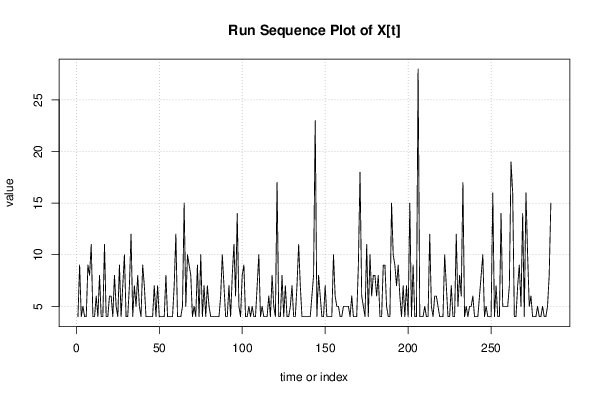
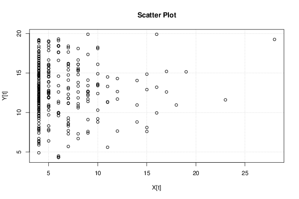
| Dataseries X: | |||||||||||||||||||||||||||||||||||||||||||||||||||||||||||||||||
4 9 4 5 4 4 9 8 11 4 4 6 4 8 4 4 11 4 4 6 6 4 8 5 4 9 4 7 10 4 4 7 12 4 7 5 8 5 4 9 7 4 4 4 4 4 7 4 7 4 4 4 4 8 4 4 4 4 7 12 4 4 4 5 15 5 10 9 8 4 5 4 9 4 10 4 7 4 7 5 4 4 4 4 4 4 6 10 7 4 4 7 4 8 11 6 14 5 4 8 9 4 4 5 4 5 4 4 7 10 4 5 4 4 4 6 4 8 5 4 17 4 4 8 4 7 4 4 5 7 4 4 7 11 7 4 4 4 4 4 4 6 8 23 4 8 6 4 4 7 4 4 4 4 10 6 5 5 4 4 5 5 5 5 4 6 4 4 4 9 18 6 5 4 11 4 10 6 8 8 6 8 4 4 9 9 5 4 4 15 10 9 7 9 6 4 7 4 7 4 15 4 9 4 4 28 4 4 4 5 4 4 12 5 4 6 6 5 4 4 4 10 7 4 4 7 4 4 12 5 8 6 17 4 5 4 5 5 6 4 4 4 6 8 10 4 5 4 4 4 16 4 7 4 4 14 5 5 5 5 7 19 16 4 4 7 9 5 14 4 16 10 5 6 4 4 4 5 4 4 5 4 4 5 8 15 | |||||||||||||||||||||||||||||||||||||||||||||||||||||||||||||||||
| Dataseries Y: | |||||||||||||||||||||||||||||||||||||||||||||||||||||||||||||||||
12,9 7,4 12,2 12,8 7,4 6,7 12,6 14,8 13,3 11,1 8,2 11,4 6,4 10,6 12,0 6,3 11,3 11,9 9,3 9,6 10,0 6,4 13,8 10,8 13,8 11,7 10,9 16,1 13,4 9,9 11,5 8,3 11,7 6,1 9,0 9,7 10,8 10,3 10,4 12,7 9,3 11,8 5,9 11,4 13,0 10,8 12,3 11,3 11,8 7,9 12,7 12,3 11,6 6,7 10,9 12,1 13,3 10,1 5,7 14,3 8,0 13,3 9,3 12,5 7,6 15,9 9,2 9,1 11,1 13,0 14,5 12,2 12,3 11,4 8,8 14,6 7,3 12,6 13,0 12,6 13,2 9,9 7,7 10,5 13,4 10,9 4,3 10,3 11,8 11,2 11,4 8,6 13,2 12,6 5,6 9,9 8,8 7,7 9,0 7,3 11,4 13,6 7,9 10,7 10,3 8,3 9,6 14,2 8,5 13,5 4,9 6,4 9,6 11,6 11,1 4,35 12,7 18,1 17,85 16,6 12,6 17,1 19,1 16,1 13,35 18,4 14,7 10,6 12,6 16,2 13,6 18,9 14,1 14,5 16,15 14,75 14,8 12,45 12,65 17,35 8,6 18,4 16,1 11,6 17,75 15,25 17,65 15,6 16,35 17,65 13,6 11,7 14,35 14,75 18,25 9,9 16 18,25 16,85 14,6 13,85 18,95 15,6 14,85 11,75 18,45 15,9 17,1 16,1 19,9 10,95 18,45 15,1 15 11,35 15,95 18,1 14,6 15,4 15,4 17,6 13,35 19,1 15,35 7,6 13,4 13,9 19,1 15,25 12,9 16,1 17,35 13,15 12,15 12,6 10,35 15,4 9,6 18,2 13,6 14,85 14,75 14,1 14,9 16,25 19,25 13,6 13,6 15,65 12,75 14,6 9,85 12,65 11,9 19,2 16,6 11,2 15,25 11,9 13,2 16,35 12,4 15,85 14,35 18,15 11,15 15,65 17,75 7,65 12,35 15,6 19,3 15,2 17,1 15,6 18,4 19,05 18,55 19,1 13,1 12,85 9,5 4,5 11,85 13,6 11,7 12,4 13,35 11,4 14,9 19,9 17,75 11,2 14,6 17,6 14,05 16,1 13,35 11,85 11,95 14,75 15,15 13,2 16,85 7,85 7,7 12,6 7,85 10,95 12,35 9,95 14,9 16,65 13,4 13,95 15,7 16,85 10,95 15,35 12,2 15,1 17,75 15,2 14,6 16,65 8,1 | |||||||||||||||||||||||||||||||||||||||||||||||||||||||||||||||||
Tables (Output of Computation) | |||||||||||||||||||||||||||||||||||||||||||||||||||||||||||||||||
| |||||||||||||||||||||||||||||||||||||||||||||||||||||||||||||||||
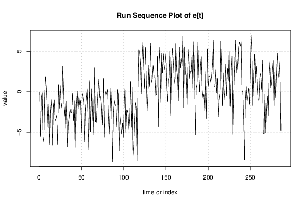
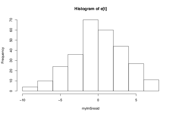
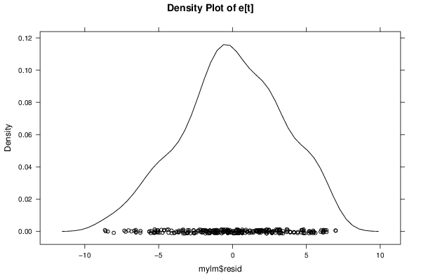
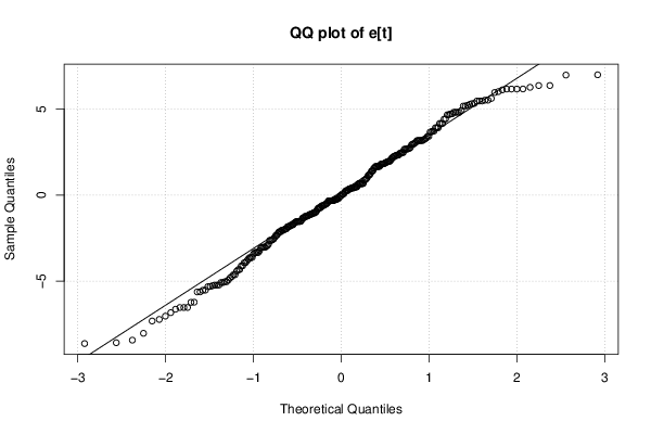
Figures (Output of Computation) | |||||||||||||||||||||||||||||||||||||||||||||||||||||||||||||||||
Input Parameters & R Code | |||||||||||||||||||||||||||||||||||||||||||||||||||||||||||||||||
| Parameters (Session): | |||||||||||||||||||||||||||||||||||||||||||||||||||||||||||||||||
| par1 = 0 ; par2 = 0 ; | |||||||||||||||||||||||||||||||||||||||||||||||||||||||||||||||||
| Parameters (R input): | |||||||||||||||||||||||||||||||||||||||||||||||||||||||||||||||||
| par1 = 0 ; par2 = 0 ; | |||||||||||||||||||||||||||||||||||||||||||||||||||||||||||||||||
| R code (references can be found in the software module): | |||||||||||||||||||||||||||||||||||||||||||||||||||||||||||||||||
par1 <- as.numeric(par1) | |||||||||||||||||||||||||||||||||||||||||||||||||||||||||||||||||