Repository of Reproducible Computations

Free Statistics

of Irreproducible Research!

Author's title

Author

*Unverified author*

R Software Module

rwasp_autocorrelation.wasp

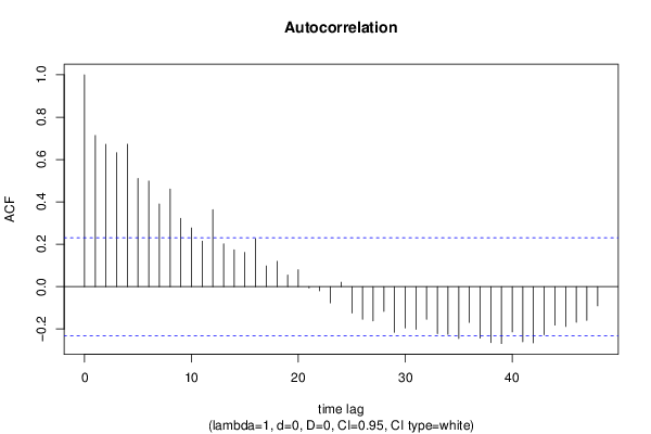
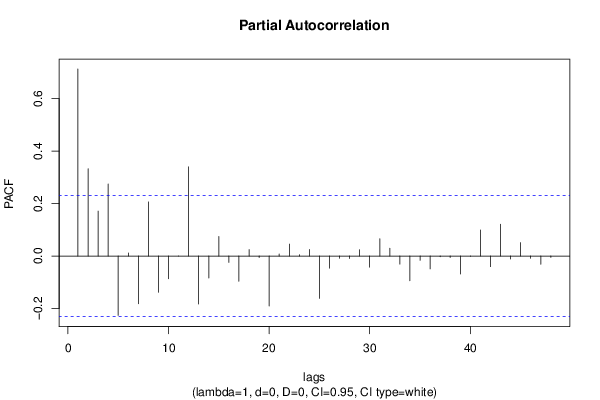
Title produced by software

(Partial) Autocorrelation Function

Date of computation

Fri, 14 Mar 2014 09:57:34 -0400

Cite this page as follows

Statistical Computations at FreeStatistics.org, Office for Research Development and Education, URL https://freestatistics.org/blog/index.php?v=date/2014/Mar/14/t1394805991tfyx030vvqso3ob.htm/, Retrieved Tue, 14 May 2024 07:44:52 +0000

Statistical Computations at FreeStatistics.org, Office for Research Development and Education, URL https://freestatistics.org/blog/index.php?pk=234246, Retrieved Tue, 14 May 2024 07:44:52 +0000

QR Codes:

Paste this QR Code to cite your computation.

Original text written by user:

IsPrivate?

No (this computation is public)

User-defined keywords

Estimated Impact

148

Family? (F = Feedback message, R = changed R code, M = changed R Module, P = changed Parameters, D = changed Data)

-     [Univariate Data Series] [] [2014-03-03 21:01:19] [967af62594a7ddaeafac2725d7422db7]
- RMP   [Mean Plot] [] [2014-03-03 21:11:19] [967af62594a7ddaeafac2725d7422db7]
- RMPD      [(Partial) Autocorrelation Function] [] [2014-03-14 13:57:34] [a051cf513b3103c0fd2487dcb9eab576] [Current]
- R P         [(Partial) Autocorrelation Function] [] [2014-03-14 15:08:55] [967af62594a7ddaeafac2725d7422db7] 
-    D          [(Partial) Autocorrelation Function] [] [2014-03-14 17:20:55] [967af62594a7ddaeafac2725d7422db7] 
-   PD        [(Partial) Autocorrelation Function] [] [2014-03-14 15:22:38] [967af62594a7ddaeafac2725d7422db7] 
- RMPD        [Mean Plot] [] [2014-03-14 16:46:30] [967af62594a7ddaeafac2725d7422db7] 

Feedback Forum

Post a new message

Dataseries X:

Download CSV

Histogram

Boxplots

Summary of computational transaction
Raw Input	view raw input (R code)
Raw Output	view raw output of R engine
Computing time	3 seconds
R Server	'Gertrude Mary Cox' @ cox.wessa.net

\begin{tabular}{lllllllll}
\hline
Summary of computational transaction \tabularnewline
Raw Input & view raw input (R code)  \tabularnewline
Raw Output & view raw output of R engine  \tabularnewline
Computing time & 3 seconds \tabularnewline
R Server & 'Gertrude Mary Cox' @ cox.wessa.net \tabularnewline
\hline
\end{tabular}
%Source: https://freestatistics.org/blog/index.php?pk=234246&T=0

[TABLE]
[ROW][C]Summary of computational transaction[/C][/ROW]
[ROW][C]Raw Input[/C][C]view raw input (R code) [/C][/ROW]
[ROW][C]Raw Output[/C][C]view raw output of R engine [/C][/ROW]
[ROW][C]Computing time[/C][C]3 seconds[/C][/ROW]
[ROW][C]R Server[/C][C]'Gertrude Mary Cox' @ cox.wessa.net[/C][/ROW]
[/TABLE]
Source: https://freestatistics.org/blog/index.php?pk=234246&T=0

Globally Unique Identifier (entire table): ba.freestatistics.org/blog/index.php?pk=234246&T=0

As an alternative you can also use a QR Code:

The GUIDs for individual cells are displayed in the table below:

Summary of computational transaction
Raw Input	view raw input (R code)
Raw Output	view raw output of R engine
Computing time	3 seconds
R Server	'Gertrude Mary Cox' @ cox.wessa.net

Autocorrelation Function
Time lag k	ACF(k)	T-STAT	P-value
1	0.713466	6.054	0
2	0.672358	5.7051	0
3	0.632282	5.3651	0
4	0.672415	5.7056	0
5	0.510457	4.3314	2.4e-05
6	0.498439	4.2294	3.4e-05
7	0.390445	3.313	0.000723
8	0.460658	3.9088	0.000104
9	0.322559	2.737	0.003903
10	0.276968	2.3501	0.010755
11	0.214604	1.821	0.036382
12	0.363444	3.0839	0.001448
13	0.202106	1.7149	0.04533
14	0.173883	1.4754	0.072226
15	0.16173	1.3723	0.087111
16	0.226129	1.9188	0.029489
17	0.097571	0.8279	0.205228
18	0.119461	1.0137	0.15707
19	0.055019	0.4669	0.321007
20	0.079759	0.6768	0.250357
21	-0.006343	-0.0538	0.478613
22	-0.019264	-0.1635	0.435306
23	-0.076768	-0.6514	0.258432
24	0.02088	0.1772	0.429935
25	-0.124324	-1.0549	0.147494
26	-0.154313	-1.3094	0.097284
27	-0.161413	-1.3696	0.087529
28	-0.117314	-0.9954	0.161428
29	-0.215931	-1.8322	0.035526
30	-0.194929	-1.654	0.051238
31	-0.201402	-1.709	0.045883
32	-0.153769	-1.3048	0.098062
33	-0.221625	-1.8806	0.032039
34	-0.225	-1.9092	0.030112
35	-0.244862	-2.0777	0.020651
36	-0.168886	-1.433	0.078086
37	-0.243061	-2.0624	0.021387
38	-0.264526	-2.2446	0.013934
39	-0.268738	-2.2803	0.012776
40	-0.213487	-1.8115	0.037117
41	-0.26047	-2.2102	0.015137
42	-0.265496	-2.2528	0.01366
43	-0.226876	-1.9251	0.029083
44	-0.181721	-1.542	0.063734
45	-0.187971	-1.595	0.057547
46	-0.168556	-1.4302	0.078486
47	-0.159519	-1.3536	0.090055
48	-0.090577	-0.7686	0.222331

\begin{tabular}{lllllllll}
\hline
Autocorrelation Function \tabularnewline
Time lag k & ACF(k) & T-STAT & P-value \tabularnewline
1 & 0.713466 & 6.054 & 0 \tabularnewline
2 & 0.672358 & 5.7051 & 0 \tabularnewline
3 & 0.632282 & 5.3651 & 0 \tabularnewline
4 & 0.672415 & 5.7056 & 0 \tabularnewline
5 & 0.510457 & 4.3314 & 2.4e-05 \tabularnewline
6 & 0.498439 & 4.2294 & 3.4e-05 \tabularnewline
7 & 0.390445 & 3.313 & 0.000723 \tabularnewline
8 & 0.460658 & 3.9088 & 0.000104 \tabularnewline
9 & 0.322559 & 2.737 & 0.003903 \tabularnewline
10 & 0.276968 & 2.3501 & 0.010755 \tabularnewline
11 & 0.214604 & 1.821 & 0.036382 \tabularnewline
12 & 0.363444 & 3.0839 & 0.001448 \tabularnewline
13 & 0.202106 & 1.7149 & 0.04533 \tabularnewline
14 & 0.173883 & 1.4754 & 0.072226 \tabularnewline
15 & 0.16173 & 1.3723 & 0.087111 \tabularnewline
16 & 0.226129 & 1.9188 & 0.029489 \tabularnewline
17 & 0.097571 & 0.8279 & 0.205228 \tabularnewline
18 & 0.119461 & 1.0137 & 0.15707 \tabularnewline
19 & 0.055019 & 0.4669 & 0.321007 \tabularnewline
20 & 0.079759 & 0.6768 & 0.250357 \tabularnewline
21 & -0.006343 & -0.0538 & 0.478613 \tabularnewline
22 & -0.019264 & -0.1635 & 0.435306 \tabularnewline
23 & -0.076768 & -0.6514 & 0.258432 \tabularnewline
24 & 0.02088 & 0.1772 & 0.429935 \tabularnewline
25 & -0.124324 & -1.0549 & 0.147494 \tabularnewline
26 & -0.154313 & -1.3094 & 0.097284 \tabularnewline
27 & -0.161413 & -1.3696 & 0.087529 \tabularnewline
28 & -0.117314 & -0.9954 & 0.161428 \tabularnewline
29 & -0.215931 & -1.8322 & 0.035526 \tabularnewline
30 & -0.194929 & -1.654 & 0.051238 \tabularnewline
31 & -0.201402 & -1.709 & 0.045883 \tabularnewline
32 & -0.153769 & -1.3048 & 0.098062 \tabularnewline
33 & -0.221625 & -1.8806 & 0.032039 \tabularnewline
34 & -0.225 & -1.9092 & 0.030112 \tabularnewline
35 & -0.244862 & -2.0777 & 0.020651 \tabularnewline
36 & -0.168886 & -1.433 & 0.078086 \tabularnewline
37 & -0.243061 & -2.0624 & 0.021387 \tabularnewline
38 & -0.264526 & -2.2446 & 0.013934 \tabularnewline
39 & -0.268738 & -2.2803 & 0.012776 \tabularnewline
40 & -0.213487 & -1.8115 & 0.037117 \tabularnewline
41 & -0.26047 & -2.2102 & 0.015137 \tabularnewline
42 & -0.265496 & -2.2528 & 0.01366 \tabularnewline
43 & -0.226876 & -1.9251 & 0.029083 \tabularnewline
44 & -0.181721 & -1.542 & 0.063734 \tabularnewline
45 & -0.187971 & -1.595 & 0.057547 \tabularnewline
46 & -0.168556 & -1.4302 & 0.078486 \tabularnewline
47 & -0.159519 & -1.3536 & 0.090055 \tabularnewline
48 & -0.090577 & -0.7686 & 0.222331 \tabularnewline
\hline
\end{tabular}
%Source: https://freestatistics.org/blog/index.php?pk=234246&T=1

[TABLE]
[ROW][C]Autocorrelation Function[/C][/ROW]
[ROW][C]Time lag k[/C][C]ACF(k)[/C][C]T-STAT[/C][C]P-value[/C][/ROW]
[ROW][C]1[/C][C]0.713466[/C][C]6.054[/C][C]0[/C][/ROW]
[ROW][C]2[/C][C]0.672358[/C][C]5.7051[/C][C]0[/C][/ROW]
[ROW][C]3[/C][C]0.632282[/C][C]5.3651[/C][C]0[/C][/ROW]
[ROW][C]4[/C][C]0.672415[/C][C]5.7056[/C][C]0[/C][/ROW]
[ROW][C]5[/C][C]0.510457[/C][C]4.3314[/C][C]2.4e-05[/C][/ROW]
[ROW][C]6[/C][C]0.498439[/C][C]4.2294[/C][C]3.4e-05[/C][/ROW]
[ROW][C]7[/C][C]0.390445[/C][C]3.313[/C][C]0.000723[/C][/ROW]
[ROW][C]8[/C][C]0.460658[/C][C]3.9088[/C][C]0.000104[/C][/ROW]
[ROW][C]9[/C][C]0.322559[/C][C]2.737[/C][C]0.003903[/C][/ROW]
[ROW][C]10[/C][C]0.276968[/C][C]2.3501[/C][C]0.010755[/C][/ROW]
[ROW][C]11[/C][C]0.214604[/C][C]1.821[/C][C]0.036382[/C][/ROW]
[ROW][C]12[/C][C]0.363444[/C][C]3.0839[/C][C]0.001448[/C][/ROW]
[ROW][C]13[/C][C]0.202106[/C][C]1.7149[/C][C]0.04533[/C][/ROW]
[ROW][C]14[/C][C]0.173883[/C][C]1.4754[/C][C]0.072226[/C][/ROW]
[ROW][C]15[/C][C]0.16173[/C][C]1.3723[/C][C]0.087111[/C][/ROW]
[ROW][C]16[/C][C]0.226129[/C][C]1.9188[/C][C]0.029489[/C][/ROW]
[ROW][C]17[/C][C]0.097571[/C][C]0.8279[/C][C]0.205228[/C][/ROW]
[ROW][C]18[/C][C]0.119461[/C][C]1.0137[/C][C]0.15707[/C][/ROW]
[ROW][C]19[/C][C]0.055019[/C][C]0.4669[/C][C]0.321007[/C][/ROW]
[ROW][C]20[/C][C]0.079759[/C][C]0.6768[/C][C]0.250357[/C][/ROW]
[ROW][C]21[/C][C]-0.006343[/C][C]-0.0538[/C][C]0.478613[/C][/ROW]
[ROW][C]22[/C][C]-0.019264[/C][C]-0.1635[/C][C]0.435306[/C][/ROW]
[ROW][C]23[/C][C]-0.076768[/C][C]-0.6514[/C][C]0.258432[/C][/ROW]
[ROW][C]24[/C][C]0.02088[/C][C]0.1772[/C][C]0.429935[/C][/ROW]
[ROW][C]25[/C][C]-0.124324[/C][C]-1.0549[/C][C]0.147494[/C][/ROW]
[ROW][C]26[/C][C]-0.154313[/C][C]-1.3094[/C][C]0.097284[/C][/ROW]
[ROW][C]27[/C][C]-0.161413[/C][C]-1.3696[/C][C]0.087529[/C][/ROW]
[ROW][C]28[/C][C]-0.117314[/C][C]-0.9954[/C][C]0.161428[/C][/ROW]
[ROW][C]29[/C][C]-0.215931[/C][C]-1.8322[/C][C]0.035526[/C][/ROW]
[ROW][C]30[/C][C]-0.194929[/C][C]-1.654[/C][C]0.051238[/C][/ROW]
[ROW][C]31[/C][C]-0.201402[/C][C]-1.709[/C][C]0.045883[/C][/ROW]
[ROW][C]32[/C][C]-0.153769[/C][C]-1.3048[/C][C]0.098062[/C][/ROW]
[ROW][C]33[/C][C]-0.221625[/C][C]-1.8806[/C][C]0.032039[/C][/ROW]
[ROW][C]34[/C][C]-0.225[/C][C]-1.9092[/C][C]0.030112[/C][/ROW]
[ROW][C]35[/C][C]-0.244862[/C][C]-2.0777[/C][C]0.020651[/C][/ROW]
[ROW][C]36[/C][C]-0.168886[/C][C]-1.433[/C][C]0.078086[/C][/ROW]
[ROW][C]37[/C][C]-0.243061[/C][C]-2.0624[/C][C]0.021387[/C][/ROW]
[ROW][C]38[/C][C]-0.264526[/C][C]-2.2446[/C][C]0.013934[/C][/ROW]
[ROW][C]39[/C][C]-0.268738[/C][C]-2.2803[/C][C]0.012776[/C][/ROW]
[ROW][C]40[/C][C]-0.213487[/C][C]-1.8115[/C][C]0.037117[/C][/ROW]
[ROW][C]41[/C][C]-0.26047[/C][C]-2.2102[/C][C]0.015137[/C][/ROW]
[ROW][C]42[/C][C]-0.265496[/C][C]-2.2528[/C][C]0.01366[/C][/ROW]
[ROW][C]43[/C][C]-0.226876[/C][C]-1.9251[/C][C]0.029083[/C][/ROW]
[ROW][C]44[/C][C]-0.181721[/C][C]-1.542[/C][C]0.063734[/C][/ROW]
[ROW][C]45[/C][C]-0.187971[/C][C]-1.595[/C][C]0.057547[/C][/ROW]
[ROW][C]46[/C][C]-0.168556[/C][C]-1.4302[/C][C]0.078486[/C][/ROW]
[ROW][C]47[/C][C]-0.159519[/C][C]-1.3536[/C][C]0.090055[/C][/ROW]
[ROW][C]48[/C][C]-0.090577[/C][C]-0.7686[/C][C]0.222331[/C][/ROW]
[/TABLE]
Source: https://freestatistics.org/blog/index.php?pk=234246&T=1

Globally Unique Identifier (entire table): ba.freestatistics.org/blog/index.php?pk=234246&T=1

As an alternative you can also use a QR Code:

The GUIDs for individual cells are displayed in the table below:

Autocorrelation Function
Time lag k	ACF(k)	T-STAT	P-value
1	0.713466	6.054	0
2	0.672358	5.7051	0
3	0.632282	5.3651	0
4	0.672415	5.7056	0
5	0.510457	4.3314	2.4e-05
6	0.498439	4.2294	3.4e-05
7	0.390445	3.313	0.000723
8	0.460658	3.9088	0.000104
9	0.322559	2.737	0.003903
10	0.276968	2.3501	0.010755
11	0.214604	1.821	0.036382
12	0.363444	3.0839	0.001448
13	0.202106	1.7149	0.04533
14	0.173883	1.4754	0.072226
15	0.16173	1.3723	0.087111
16	0.226129	1.9188	0.029489
17	0.097571	0.8279	0.205228
18	0.119461	1.0137	0.15707
19	0.055019	0.4669	0.321007
20	0.079759	0.6768	0.250357
21	-0.006343	-0.0538	0.478613
22	-0.019264	-0.1635	0.435306
23	-0.076768	-0.6514	0.258432
24	0.02088	0.1772	0.429935
25	-0.124324	-1.0549	0.147494
26	-0.154313	-1.3094	0.097284
27	-0.161413	-1.3696	0.087529
28	-0.117314	-0.9954	0.161428
29	-0.215931	-1.8322	0.035526
30	-0.194929	-1.654	0.051238
31	-0.201402	-1.709	0.045883
32	-0.153769	-1.3048	0.098062
33	-0.221625	-1.8806	0.032039
34	-0.225	-1.9092	0.030112
35	-0.244862	-2.0777	0.020651
36	-0.168886	-1.433	0.078086
37	-0.243061	-2.0624	0.021387
38	-0.264526	-2.2446	0.013934
39	-0.268738	-2.2803	0.012776
40	-0.213487	-1.8115	0.037117
41	-0.26047	-2.2102	0.015137
42	-0.265496	-2.2528	0.01366
43	-0.226876	-1.9251	0.029083
44	-0.181721	-1.542	0.063734
45	-0.187971	-1.595	0.057547
46	-0.168556	-1.4302	0.078486
47	-0.159519	-1.3536	0.090055
48	-0.090577	-0.7686	0.222331

Partial Autocorrelation Function
Time lag k	PACF(k)	T-STAT	P-value
1	0.713466	6.054	0
2	0.33266	2.8227	0.003076
3	0.171343	1.4539	0.07516
4	0.274523	2.3294	0.011323
5	-0.226138	-1.9188	0.029484
6	0.01165	0.0989	0.460763
7	-0.181846	-1.543	0.063606
8	0.20656	1.7527	0.041953
9	-0.137819	-1.1694	0.123043
10	-0.08621	-0.7315	0.233418
11	-2.4e-05	-2e-04	0.49992
12	0.340195	2.8867	0.002568
13	-0.183011	-1.5529	0.062415
14	-0.083862	-0.7116	0.239509
15	0.074589	0.6329	0.264399
16	-0.024028	-0.2039	0.419509
17	-0.095809	-0.813	0.209458
18	0.024762	0.2101	0.417087
19	-0.005221	-0.0443	0.482393
20	-0.190341	-1.6151	0.055332
21	0.008176	0.0694	0.472441
22	0.045515	0.3862	0.350242
23	0.005125	0.0435	0.482718
24	0.025253	0.2143	0.415469
25	-0.161486	-1.3703	0.087433
26	-0.046075	-0.391	0.348492
27	-0.008669	-0.0736	0.470784
28	-0.008979	-0.0762	0.46974
29	0.024109	0.2046	0.419243
30	-0.042324	-0.3591	0.360274
31	0.065928	0.5594	0.288807
32	0.030103	0.2554	0.399558
33	-0.030809	-0.2614	0.397256
34	-0.094442	-0.8014	0.212778
35	-0.016326	-0.1385	0.445104
36	-0.048798	-0.4141	0.340028
37	-0.002598	-0.022	0.491237
38	-0.00545	-0.0462	0.481622
39	-0.068401	-0.5804	0.281727
40	-0.000896	-0.0076	0.496979
41	0.099668	0.8457	0.200258
42	-0.040339	-0.3423	0.366565
43	0.121284	1.0291	0.153432
44	-0.011472	-0.0973	0.461363
45	0.051321	0.4355	0.332261
46	-0.008594	-0.0729	0.471035
47	-0.030947	-0.2626	0.396806
48	-0.005113	-0.0434	0.482758

\begin{tabular}{lllllllll}
\hline
Partial Autocorrelation Function \tabularnewline
Time lag k & PACF(k) & T-STAT & P-value \tabularnewline
1 & 0.713466 & 6.054 & 0 \tabularnewline
2 & 0.33266 & 2.8227 & 0.003076 \tabularnewline
3 & 0.171343 & 1.4539 & 0.07516 \tabularnewline
4 & 0.274523 & 2.3294 & 0.011323 \tabularnewline
5 & -0.226138 & -1.9188 & 0.029484 \tabularnewline
6 & 0.01165 & 0.0989 & 0.460763 \tabularnewline
7 & -0.181846 & -1.543 & 0.063606 \tabularnewline
8 & 0.20656 & 1.7527 & 0.041953 \tabularnewline
9 & -0.137819 & -1.1694 & 0.123043 \tabularnewline
10 & -0.08621 & -0.7315 & 0.233418 \tabularnewline
11 & -2.4e-05 & -2e-04 & 0.49992 \tabularnewline
12 & 0.340195 & 2.8867 & 0.002568 \tabularnewline
13 & -0.183011 & -1.5529 & 0.062415 \tabularnewline
14 & -0.083862 & -0.7116 & 0.239509 \tabularnewline
15 & 0.074589 & 0.6329 & 0.264399 \tabularnewline
16 & -0.024028 & -0.2039 & 0.419509 \tabularnewline
17 & -0.095809 & -0.813 & 0.209458 \tabularnewline
18 & 0.024762 & 0.2101 & 0.417087 \tabularnewline
19 & -0.005221 & -0.0443 & 0.482393 \tabularnewline
20 & -0.190341 & -1.6151 & 0.055332 \tabularnewline
21 & 0.008176 & 0.0694 & 0.472441 \tabularnewline
22 & 0.045515 & 0.3862 & 0.350242 \tabularnewline
23 & 0.005125 & 0.0435 & 0.482718 \tabularnewline
24 & 0.025253 & 0.2143 & 0.415469 \tabularnewline
25 & -0.161486 & -1.3703 & 0.087433 \tabularnewline
26 & -0.046075 & -0.391 & 0.348492 \tabularnewline
27 & -0.008669 & -0.0736 & 0.470784 \tabularnewline
28 & -0.008979 & -0.0762 & 0.46974 \tabularnewline
29 & 0.024109 & 0.2046 & 0.419243 \tabularnewline
30 & -0.042324 & -0.3591 & 0.360274 \tabularnewline
31 & 0.065928 & 0.5594 & 0.288807 \tabularnewline
32 & 0.030103 & 0.2554 & 0.399558 \tabularnewline
33 & -0.030809 & -0.2614 & 0.397256 \tabularnewline
34 & -0.094442 & -0.8014 & 0.212778 \tabularnewline
35 & -0.016326 & -0.1385 & 0.445104 \tabularnewline
36 & -0.048798 & -0.4141 & 0.340028 \tabularnewline
37 & -0.002598 & -0.022 & 0.491237 \tabularnewline
38 & -0.00545 & -0.0462 & 0.481622 \tabularnewline
39 & -0.068401 & -0.5804 & 0.281727 \tabularnewline
40 & -0.000896 & -0.0076 & 0.496979 \tabularnewline
41 & 0.099668 & 0.8457 & 0.200258 \tabularnewline
42 & -0.040339 & -0.3423 & 0.366565 \tabularnewline
43 & 0.121284 & 1.0291 & 0.153432 \tabularnewline
44 & -0.011472 & -0.0973 & 0.461363 \tabularnewline
45 & 0.051321 & 0.4355 & 0.332261 \tabularnewline
46 & -0.008594 & -0.0729 & 0.471035 \tabularnewline
47 & -0.030947 & -0.2626 & 0.396806 \tabularnewline
48 & -0.005113 & -0.0434 & 0.482758 \tabularnewline
\hline
\end{tabular}
%Source: https://freestatistics.org/blog/index.php?pk=234246&T=2

[TABLE]
[ROW][C]Partial Autocorrelation Function[/C][/ROW]
[ROW][C]Time lag k[/C][C]PACF(k)[/C][C]T-STAT[/C][C]P-value[/C][/ROW]
[ROW][C]1[/C][C]0.713466[/C][C]6.054[/C][C]0[/C][/ROW]
[ROW][C]2[/C][C]0.33266[/C][C]2.8227[/C][C]0.003076[/C][/ROW]
[ROW][C]3[/C][C]0.171343[/C][C]1.4539[/C][C]0.07516[/C][/ROW]
[ROW][C]4[/C][C]0.274523[/C][C]2.3294[/C][C]0.011323[/C][/ROW]
[ROW][C]5[/C][C]-0.226138[/C][C]-1.9188[/C][C]0.029484[/C][/ROW]
[ROW][C]6[/C][C]0.01165[/C][C]0.0989[/C][C]0.460763[/C][/ROW]
[ROW][C]7[/C][C]-0.181846[/C][C]-1.543[/C][C]0.063606[/C][/ROW]
[ROW][C]8[/C][C]0.20656[/C][C]1.7527[/C][C]0.041953[/C][/ROW]
[ROW][C]9[/C][C]-0.137819[/C][C]-1.1694[/C][C]0.123043[/C][/ROW]
[ROW][C]10[/C][C]-0.08621[/C][C]-0.7315[/C][C]0.233418[/C][/ROW]
[ROW][C]11[/C][C]-2.4e-05[/C][C]-2e-04[/C][C]0.49992[/C][/ROW]
[ROW][C]12[/C][C]0.340195[/C][C]2.8867[/C][C]0.002568[/C][/ROW]
[ROW][C]13[/C][C]-0.183011[/C][C]-1.5529[/C][C]0.062415[/C][/ROW]
[ROW][C]14[/C][C]-0.083862[/C][C]-0.7116[/C][C]0.239509[/C][/ROW]
[ROW][C]15[/C][C]0.074589[/C][C]0.6329[/C][C]0.264399[/C][/ROW]
[ROW][C]16[/C][C]-0.024028[/C][C]-0.2039[/C][C]0.419509[/C][/ROW]
[ROW][C]17[/C][C]-0.095809[/C][C]-0.813[/C][C]0.209458[/C][/ROW]
[ROW][C]18[/C][C]0.024762[/C][C]0.2101[/C][C]0.417087[/C][/ROW]
[ROW][C]19[/C][C]-0.005221[/C][C]-0.0443[/C][C]0.482393[/C][/ROW]
[ROW][C]20[/C][C]-0.190341[/C][C]-1.6151[/C][C]0.055332[/C][/ROW]
[ROW][C]21[/C][C]0.008176[/C][C]0.0694[/C][C]0.472441[/C][/ROW]
[ROW][C]22[/C][C]0.045515[/C][C]0.3862[/C][C]0.350242[/C][/ROW]
[ROW][C]23[/C][C]0.005125[/C][C]0.0435[/C][C]0.482718[/C][/ROW]
[ROW][C]24[/C][C]0.025253[/C][C]0.2143[/C][C]0.415469[/C][/ROW]
[ROW][C]25[/C][C]-0.161486[/C][C]-1.3703[/C][C]0.087433[/C][/ROW]
[ROW][C]26[/C][C]-0.046075[/C][C]-0.391[/C][C]0.348492[/C][/ROW]
[ROW][C]27[/C][C]-0.008669[/C][C]-0.0736[/C][C]0.470784[/C][/ROW]
[ROW][C]28[/C][C]-0.008979[/C][C]-0.0762[/C][C]0.46974[/C][/ROW]
[ROW][C]29[/C][C]0.024109[/C][C]0.2046[/C][C]0.419243[/C][/ROW]
[ROW][C]30[/C][C]-0.042324[/C][C]-0.3591[/C][C]0.360274[/C][/ROW]
[ROW][C]31[/C][C]0.065928[/C][C]0.5594[/C][C]0.288807[/C][/ROW]
[ROW][C]32[/C][C]0.030103[/C][C]0.2554[/C][C]0.399558[/C][/ROW]
[ROW][C]33[/C][C]-0.030809[/C][C]-0.2614[/C][C]0.397256[/C][/ROW]
[ROW][C]34[/C][C]-0.094442[/C][C]-0.8014[/C][C]0.212778[/C][/ROW]
[ROW][C]35[/C][C]-0.016326[/C][C]-0.1385[/C][C]0.445104[/C][/ROW]
[ROW][C]36[/C][C]-0.048798[/C][C]-0.4141[/C][C]0.340028[/C][/ROW]
[ROW][C]37[/C][C]-0.002598[/C][C]-0.022[/C][C]0.491237[/C][/ROW]
[ROW][C]38[/C][C]-0.00545[/C][C]-0.0462[/C][C]0.481622[/C][/ROW]
[ROW][C]39[/C][C]-0.068401[/C][C]-0.5804[/C][C]0.281727[/C][/ROW]
[ROW][C]40[/C][C]-0.000896[/C][C]-0.0076[/C][C]0.496979[/C][/ROW]
[ROW][C]41[/C][C]0.099668[/C][C]0.8457[/C][C]0.200258[/C][/ROW]
[ROW][C]42[/C][C]-0.040339[/C][C]-0.3423[/C][C]0.366565[/C][/ROW]
[ROW][C]43[/C][C]0.121284[/C][C]1.0291[/C][C]0.153432[/C][/ROW]
[ROW][C]44[/C][C]-0.011472[/C][C]-0.0973[/C][C]0.461363[/C][/ROW]
[ROW][C]45[/C][C]0.051321[/C][C]0.4355[/C][C]0.332261[/C][/ROW]
[ROW][C]46[/C][C]-0.008594[/C][C]-0.0729[/C][C]0.471035[/C][/ROW]
[ROW][C]47[/C][C]-0.030947[/C][C]-0.2626[/C][C]0.396806[/C][/ROW]
[ROW][C]48[/C][C]-0.005113[/C][C]-0.0434[/C][C]0.482758[/C][/ROW]
[/TABLE]
Source: https://freestatistics.org/blog/index.php?pk=234246&T=2

Globally Unique Identifier (entire table): ba.freestatistics.org/blog/index.php?pk=234246&T=2

As an alternative you can also use a QR Code:

The GUIDs for individual cells are displayed in the table below:

Partial Autocorrelation Function
Time lag k	PACF(k)	T-STAT	P-value
1	0.713466	6.054	0
2	0.33266	2.8227	0.003076
3	0.171343	1.4539	0.07516
4	0.274523	2.3294	0.011323
5	-0.226138	-1.9188	0.029484
6	0.01165	0.0989	0.460763
7	-0.181846	-1.543	0.063606
8	0.20656	1.7527	0.041953
9	-0.137819	-1.1694	0.123043
10	-0.08621	-0.7315	0.233418
11	-2.4e-05	-2e-04	0.49992
12	0.340195	2.8867	0.002568
13	-0.183011	-1.5529	0.062415
14	-0.083862	-0.7116	0.239509
15	0.074589	0.6329	0.264399
16	-0.024028	-0.2039	0.419509
17	-0.095809	-0.813	0.209458
18	0.024762	0.2101	0.417087
19	-0.005221	-0.0443	0.482393
20	-0.190341	-1.6151	0.055332
21	0.008176	0.0694	0.472441
22	0.045515	0.3862	0.350242
23	0.005125	0.0435	0.482718
24	0.025253	0.2143	0.415469
25	-0.161486	-1.3703	0.087433
26	-0.046075	-0.391	0.348492
27	-0.008669	-0.0736	0.470784
28	-0.008979	-0.0762	0.46974
29	0.024109	0.2046	0.419243
30	-0.042324	-0.3591	0.360274
31	0.065928	0.5594	0.288807
32	0.030103	0.2554	0.399558
33	-0.030809	-0.2614	0.397256
34	-0.094442	-0.8014	0.212778
35	-0.016326	-0.1385	0.445104
36	-0.048798	-0.4141	0.340028
37	-0.002598	-0.022	0.491237
38	-0.00545	-0.0462	0.481622
39	-0.068401	-0.5804	0.281727
40	-0.000896	-0.0076	0.496979
41	0.099668	0.8457	0.200258
42	-0.040339	-0.3423	0.366565
43	0.121284	1.0291	0.153432
44	-0.011472	-0.0973	0.461363
45	0.051321	0.4355	0.332261
46	-0.008594	-0.0729	0.471035
47	-0.030947	-0.2626	0.396806
48	-0.005113	-0.0434	0.482758

Figure 1

PNG link

Postscript link

PDF link

Figure 2

PNG link

Postscript link

PDF link

Figure 3

PNG link

Postscript link

PDF link

Parameters (Session):

par1 = 48 ; par2 = 1 ; par3 = 0 ; par4 = 0 ; par5 = 12 ; par6 = White Noise ; par7 = 0.95 ;

Parameters (R input):

par1 = 48 ; par2 = 1 ; par3 = 0 ; par4 = 0 ; par5 = 12 ; par6 = White Noise ; par7 = 0.95 ; par8 = ;

R code (references can be found in the software module):

if (par1 == 'Default') {
par1 = 10*log10(length(x))
} else {
par1 <- as.numeric(par1)
}
par2 <- as.numeric(par2)
par3 <- as.numeric(par3)
par4 <- as.numeric(par4)
par5 <- as.numeric(par5)
if (par6 == 'White Noise') par6 <- 'white' else par6 <- 'ma'
par7 <- as.numeric(par7)
if (par8 != '') par8 <- as.numeric(par8)
ox <- x
if (par8 == '') {
if (par2 == 0) {
x <- log(x)
} else {
x <- (x ^ par2 - 1) / par2
}
} else {
x <- log(x,base=par8)
}
if (par3 > 0) x <- diff(x,lag=1,difference=par3)
if (par4 > 0) x <- diff(x,lag=par5,difference=par4)
bitmap(file='picts.png')
op <- par(mfrow=c(2,1))
plot(ox,type='l',main='Original Time Series',xlab='time',ylab='value')
if (par8=='') {
mytitle <- paste('Working Time Series (lambda=',par2,', d=',par3,', D=',par4,')',sep='')
mysub <- paste('(lambda=',par2,', d=',par3,', D=',par4,', CI=', par7, ', CI type=',par6,')',sep='')
} else {
mytitle <- paste('Working Time Series (base=',par8,', d=',par3,', D=',par4,')',sep='')
mysub <- paste('(base=',par8,', d=',par3,', D=',par4,', CI=', par7, ', CI type=',par6,')',sep='')
}
plot(x,type='l', main=mytitle,xlab='time',ylab='value')
par(op)
dev.off()
bitmap(file='pic1.png')
racf <- acf(x, par1, main='Autocorrelation', xlab='time lag', ylab='ACF', ci.type=par6, ci=par7, sub=mysub)
dev.off()
bitmap(file='pic2.png')
rpacf <- pacf(x,par1,main='Partial Autocorrelation',xlab='lags',ylab='PACF',sub=mysub)
dev.off()
(myacf <- c(racf$acf))
(mypacf <- c(rpacf$acf))
lengthx <- length(x)
sqrtn <- sqrt(lengthx)
load(file='createtable')
a<-table.start()
a<-table.row.start(a)
a<-table.element(a,'Autocorrelation Function',4,TRUE)
a<-table.row.end(a)
a<-table.row.start(a)
a<-table.element(a,'Time lag k',header=TRUE)
a<-table.element(a,hyperlink('basics.htm','ACF(k)','click here for more information about the Autocorrelation Function'),header=TRUE)
a<-table.element(a,'T-STAT',header=TRUE)
a<-table.element(a,'P-value',header=TRUE)
a<-table.row.end(a)
for (i in 2:(par1+1)) {
a<-table.row.start(a)
a<-table.element(a,i-1,header=TRUE)
a<-table.element(a,round(myacf[i],6))
mytstat <- myacf[i]*sqrtn
a<-table.element(a,round(mytstat,4))
a<-table.element(a,round(1-pt(abs(mytstat),lengthx),6))
a<-table.row.end(a)
}
a<-table.end(a)
table.save(a,file='mytable.tab')
a<-table.start()
a<-table.row.start(a)
a<-table.element(a,'Partial Autocorrelation Function',4,TRUE)
a<-table.row.end(a)
a<-table.row.start(a)
a<-table.element(a,'Time lag k',header=TRUE)
a<-table.element(a,hyperlink('basics.htm','PACF(k)','click here for more information about the Partial Autocorrelation Function'),header=TRUE)
a<-table.element(a,'T-STAT',header=TRUE)
a<-table.element(a,'P-value',header=TRUE)
a<-table.row.end(a)
for (i in 1:par1) {
a<-table.row.start(a)
a<-table.element(a,i,header=TRUE)
a<-table.element(a,round(mypacf[i],6))
mytstat <- mypacf[i]*sqrtn
a<-table.element(a,round(mytstat,4))
a<-table.element(a,round(1-pt(abs(mytstat),lengthx),6))
a<-table.row.end(a)
}
a<-table.end(a)
table.save(a,file='mytable1.tab')

Free Statistics

Description of Statistical Computation

Tree of Dependent Computations

Dataset

Tables (Output of Computation)

Figures (Output of Computation)

Input Parameters & R Code