Repository of Reproducible Computations

Free Statistics

of Irreproducible Research!

Author's title

Author

*Unverified author*

R Software Module

rwasp_meanplot.wasp

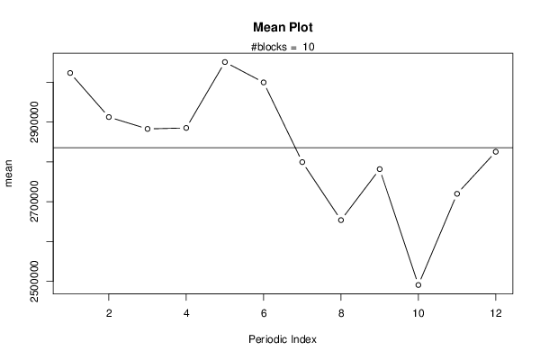
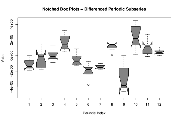
Title produced by software

Mean Plot

Date of computation

Fri, 07 Aug 2015 15:19:08 +0100

Cite this page as follows

Statistical Computations at FreeStatistics.org, Office for Research Development and Education, URL https://freestatistics.org/blog/index.php?v=date/2015/Aug/07/t1438957242xll10hujgy5ifaq.htm/, Retrieved Wed, 15 May 2024 22:40:50 +0000

Statistical Computations at FreeStatistics.org, Office for Research Development and Education, URL https://freestatistics.org/blog/index.php?pk=279902, Retrieved Wed, 15 May 2024 22:40:50 +0000

QR Codes:

Paste this QR Code to cite your computation.

Original text written by user:

IsPrivate?

No (this computation is public)

User-defined keywords

Mean plot Reeks A Sebastiaan Lunders Mercedes A-klasse omzet Ottevaere

Estimated Impact

148

Family? (F = Feedback message, R = changed R code, M = changed R Module, P = changed Parameters, D = changed Data)

-     [Univariate Data Series] [Cijferreeks A 2de...] [2015-08-05 23:58:24] [039d3b62ab99f9eeb4c9cc4c099c66fc]
- RMP   [Kernel Density Estimation] [Dichtheidsgrafiek...] [2015-08-06 13:05:13] [039d3b62ab99f9eeb4c9cc4c099c66fc]
- RMP     [Notched Boxplots] [Notched Boxplots ...] [2015-08-06 15:26:45] [039d3b62ab99f9eeb4c9cc4c099c66fc]
- RMP       [Harrell-Davis Quantiles] [Decielen Reeks A ...] [2015-08-07 12:40:19] [039d3b62ab99f9eeb4c9cc4c099c66fc]
- R P         [Harrell-Davis Quantiles] [Percentielen Reek...] [2015-08-07 13:03:56] [039d3b62ab99f9eeb4c9cc4c099c66fc]
- RMP           [Central Tendency] [Central tendency ...] [2015-08-07 14:01:29] [039d3b62ab99f9eeb4c9cc4c099c66fc]
- RMP               [Mean Plot] [Mean plot Reeks A...] [2015-08-07 14:19:08] [2cf7618d5ff65529ef2e27cea5366de0] [Current]

Feedback Forum

Post a new message

Dataseries X:

Download CSV

Histogram

Boxplots

Summary of computational transaction
Raw Input	view raw input (R code)
Raw Output	view raw output of R engine
Computing time	3 seconds
R Server	'Sir Maurice George Kendall' @ kendall.wessa.net

\begin{tabular}{lllllllll}
\hline
Summary of computational transaction \tabularnewline
Raw Input & view raw input (R code)  \tabularnewline
Raw Output & view raw output of R engine  \tabularnewline
Computing time & 3 seconds \tabularnewline
R Server & 'Sir Maurice George Kendall' @ kendall.wessa.net \tabularnewline
\hline
\end{tabular}
%Source: https://freestatistics.org/blog/index.php?pk=279902&T=0

[TABLE]
[ROW][C]Summary of computational transaction[/C][/ROW]
[ROW][C]Raw Input[/C][C]view raw input (R code) [/C][/ROW]
[ROW][C]Raw Output[/C][C]view raw output of R engine [/C][/ROW]
[ROW][C]Computing time[/C][C]3 seconds[/C][/ROW]
[ROW][C]R Server[/C][C]'Sir Maurice George Kendall' @ kendall.wessa.net[/C][/ROW]
[/TABLE]
Source: https://freestatistics.org/blog/index.php?pk=279902&T=0

Globally Unique Identifier (entire table): ba.freestatistics.org/blog/index.php?pk=279902&T=0

As an alternative you can also use a QR Code:

The GUIDs for individual cells are displayed in the table below:

Summary of computational transaction
Raw Input	view raw input (R code)
Raw Output	view raw output of R engine
Computing time	3 seconds
R Server	'Sir Maurice George Kendall' @ kendall.wessa.net

Figure 1

PNG link

Postscript link

PDF link

Figure 2

PNG link

Postscript link

PDF link

Figure 3

PNG link

Postscript link

PDF link

Figure 4

PNG link

Postscript link

PDF link

Figure 5

PNG link

Postscript link

PDF link

Figure 6

PNG link

Postscript link

PDF link

Figure 7

PNG link

Postscript link

PDF link

Parameters (Session):

par1 = 12 ;

Parameters (R input):

par1 = 12 ;

R code (references can be found in the software module):

par1 <- as.numeric(par1)
(n <- length(x))
(np <- floor(n / par1))
arr <- array(NA,dim=c(par1,np+1))
darr <- array(NA,dim=c(par1,np+1))
ari <- array(0,dim=par1)
dx <- diff(x)
j <- 0
for (i in 1:n)
{
j = j + 1
ari[j] = ari[j] + 1
arr[j,ari[j]] <- x[i]
darr[j,ari[j]] <- dx[i]
if (j == par1) j = 0
}
ari
arr
darr
arr.mean <- array(NA,dim=par1)
arr.median <- array(NA,dim=par1)
arr.midrange <- array(NA,dim=par1)
for (j in 1:par1)
{
arr.mean[j] <- mean(arr[j,],na.rm=TRUE)
arr.median[j] <- median(arr[j,],na.rm=TRUE)
arr.midrange[j] <- (quantile(arr[j,],0.75,na.rm=TRUE) + quantile(arr[j,],0.25,na.rm=TRUE)) / 2
}
overall.mean <- mean(x)
overall.median <- median(x)
overall.midrange <- (quantile(x,0.75) + quantile(x,0.25)) / 2
bitmap(file='plot1.png')
plot(arr.mean,type='b',ylab='mean',main='Mean Plot',xlab='Periodic Index')
mtext(paste('#blocks = ',np))
abline(overall.mean,0)
dev.off()
bitmap(file='plot2.png')
plot(arr.median,type='b',ylab='median',main='Median Plot',xlab='Periodic Index')
mtext(paste('#blocks = ',np))
abline(overall.median,0)
dev.off()
bitmap(file='plot3.png')
plot(arr.midrange,type='b',ylab='midrange',main='Midrange Plot',xlab='Periodic Index')
mtext(paste('#blocks = ',np))
abline(overall.midrange,0)
dev.off()
bitmap(file='plot4.png')
z <- data.frame(t(arr))
names(z) <- c(1:par1)
(boxplot(z,notch=TRUE,col='grey',xlab='Periodic Index',ylab='Value',main='Notched Box Plots - Periodic Subseries'))
dev.off()
bitmap(file='plot4b.png')
z <- data.frame(t(darr))
names(z) <- c(1:par1)
(boxplot(z,notch=TRUE,col='grey',xlab='Periodic Index',ylab='Value',main='Notched Box Plots - Differenced Periodic Subseries'))
dev.off()
bitmap(file='plot5.png')
z <- data.frame(arr)
names(z) <- c(1:np)
(boxplot(z,notch=TRUE,col='grey',xlab='Block Index',ylab='Value',main='Notched Box Plots - Sequential Blocks'))
dev.off()
bitmap(file='plot6.png')
z <- data.frame(cbind(arr.mean,arr.median,arr.midrange))
names(z) <- list('mean','median','midrange')
(boxplot(z,notch=TRUE,col='grey',ylab='Overall Central Tendency',main='Notched Box Plots'))
dev.off()

Free Statistics

Description of Statistical Computation

Tree of Dependent Computations

Dataset

Tables (Output of Computation)

Figures (Output of Computation)

Input Parameters & R Code