Free Statistics
of Irreproducible Research!
Description of Statistical Computation | |||||||||||||||||||||
|---|---|---|---|---|---|---|---|---|---|---|---|---|---|---|---|---|---|---|---|---|---|
| Author's title | |||||||||||||||||||||
| Author | *Unverified author* | ||||||||||||||||||||
| R Software Module | rwasp_meanplot.wasp | ||||||||||||||||||||
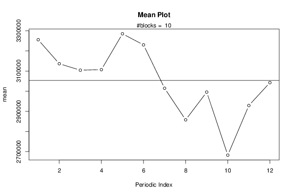
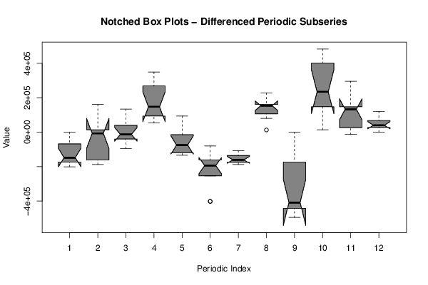
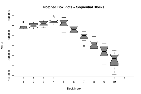
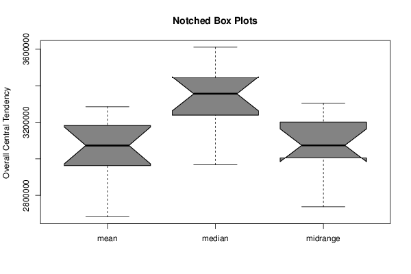
| Title produced by software | Mean Plot | ||||||||||||||||||||
| Date of computation | Fri, 07 Aug 2015 15:32:20 +0100 | ||||||||||||||||||||
| Cite this page as follows | Statistical Computations at FreeStatistics.org, Office for Research Development and Education, URL https://freestatistics.org/blog/index.php?v=date/2015/Aug/07/t1438957954m84t4cbjfh4hqo6.htm/, Retrieved Wed, 15 May 2024 09:32:16 +0000 | ||||||||||||||||||||
| Statistical Computations at FreeStatistics.org, Office for Research Development and Education, URL https://freestatistics.org/blog/index.php?pk=279903, Retrieved Wed, 15 May 2024 09:32:16 +0000 | |||||||||||||||||||||
| QR Codes: | |||||||||||||||||||||
|
| |||||||||||||||||||||
| Original text written by user: | |||||||||||||||||||||
| IsPrivate? | No (this computation is public) | ||||||||||||||||||||
| User-defined keywords | |||||||||||||||||||||
| Estimated Impact | 210 | ||||||||||||||||||||
Tree of Dependent Computations | |||||||||||||||||||||
| Family? (F = Feedback message, R = changed R code, M = changed R Module, P = changed Parameters, D = changed Data) | |||||||||||||||||||||
| - [Notched Boxplots] [] [2014-10-04 09:51:16] [3d50c3f1d1505d45371c80c331b9aa00] - D [Notched Boxplots] [] [2015-08-03 11:42:45] [74be16979710d4c4e7c6647856088456] - RMP [Harrell-Davis Quantiles] [] [2015-08-07 13:17:48] [74be16979710d4c4e7c6647856088456] - R [Harrell-Davis Quantiles] [] [2015-08-07 13:20:06] [74be16979710d4c4e7c6647856088456] - RMP [Mean Plot] [] [2015-08-07 14:32:20] [d41d8cd98f00b204e9800998ecf8427e] [Current] - RMP [(Partial) Autocorrelation Function] [] [2015-08-07 15:26:33] [74be16979710d4c4e7c6647856088456] - RMP [(Partial) Autocorrelation Function] [] [2015-08-07 16:00:37] [74be16979710d4c4e7c6647856088456] - RM [Standard Deviation Plot] [] [2015-08-07 16:22:43] [74be16979710d4c4e7c6647856088456] - RM [Standard Deviation-Mean Plot] [] [2015-08-07 16:54:54] [74be16979710d4c4e7c6647856088456] - RMP [Classical Decomposition] [] [2015-08-10 06:43:53] [74be16979710d4c4e7c6647856088456] - RMP [Exponential Smoothing] [] [2015-08-10 06:56:42] [74be16979710d4c4e7c6647856088456] - RMPD [Univariate Data Series] [] [2015-08-10 07:12:59] [74be16979710d4c4e7c6647856088456] | |||||||||||||||||||||
| Feedback Forum | |||||||||||||||||||||
Post a new message | |||||||||||||||||||||
Dataset | |||||||||||||||||||||
| Dataseries X: | |||||||||||||||||||||
3469648.00 3456726.00 3443622.00 3416504.00 3684772.00 3670576.00 3469648.00 3336060.00 3348982.00 3348982.00 3363360.00 3389204.00 3429426.00 3429426.00 3403582.00 3336060.00 3684772.00 3737916.00 3657654.00 3469648.00 3550092.00 3429426.00 3483844.00 3509870.00 3536988.00 3469648.00 3483844.00 3389204.00 3684772.00 3778138.00 3697876.00 3550092.00 3710798.00 3536988.00 3697876.00 3684772.00 3724994.00 3577210.00 3737916.00 3724994.00 3966144.00 3911726.00 3697876.00 3590132.00 3737916.00 3536988.00 3684772.00 3710798.00 3765216.00 3644732.00 3710798.00 3751020.00 3898804.00 3778138.00 3617432.00 3443622.00 3604510.00 3162250.00 3376282.00 3496766.00 3617432.00 3443622.00 3443622.00 3443622.00 3536988.00 3403582.00 3228498.00 3081988.00 3188276.00 2773316.00 3027570.00 3175354.00 3202472.00 3054688.00 3067610.00 3027570.00 3162250.00 3067610.00 2881060.00 2746198.00 2974244.00 2479022.00 2800616.00 2947126.00 2947126.00 2773316.00 2612610.00 2599688.00 2746198.00 2612610.00 2358538.00 2183454.00 2371460.00 1929382.00 2331238.00 2545088.00 2612610.00 2464826.00 2278094.00 2411682.00 2464826.00 2424604.00 2022566.00 1836016.00 1969422.00 1567566.00 1982526.00 2130310.00 2250794.00 2049866.00 1861860.00 1969422.00 2022566.00 1916278.00 1514422.00 1339338.00 1500044.00 1057966.00 1540266.00 1836016.00 | |||||||||||||||||||||
Tables (Output of Computation) | |||||||||||||||||||||
| |||||||||||||||||||||
Figures (Output of Computation) | |||||||||||||||||||||
Input Parameters & R Code | |||||||||||||||||||||
| Parameters (Session): | |||||||||||||||||||||
| par1 = 12 ; | |||||||||||||||||||||
| Parameters (R input): | |||||||||||||||||||||
| par1 = 12 ; | |||||||||||||||||||||
| R code (references can be found in the software module): | |||||||||||||||||||||
par1 <- as.numeric(par1) | |||||||||||||||||||||