Repository of Reproducible Computations

Free Statistics

of Irreproducible Research!

Author's title

Author

*Unverified author*

R Software Module

rwasp_autocorrelation.wasp

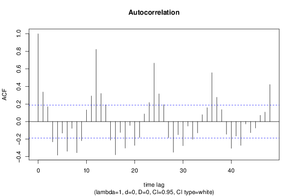
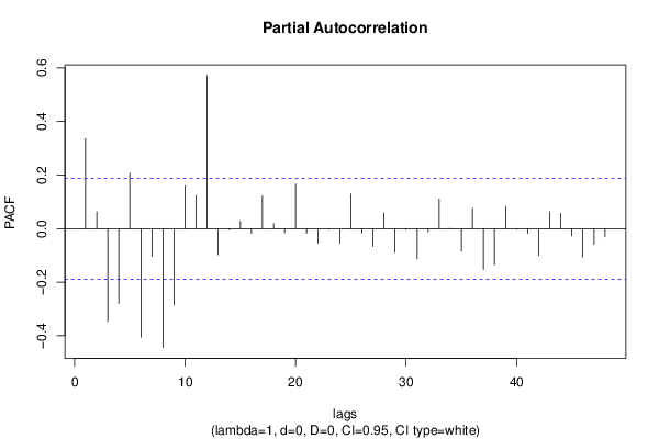
Title produced by software

(Partial) Autocorrelation Function

Date of computation

Sat, 08 Aug 2015 16:43:39 +0100

Cite this page as follows

Statistical Computations at FreeStatistics.org, Office for Research Development and Education, URL https://freestatistics.org/blog/index.php?v=date/2015/Aug/08/t14390488790jn9v4fgnlx1q5p.htm/, Retrieved Wed, 15 May 2024 15:52:11 +0000

Statistical Computations at FreeStatistics.org, Office for Research Development and Education, URL https://freestatistics.org/blog/index.php?pk=279950, Retrieved Wed, 15 May 2024 15:52:11 +0000

QR Codes:

Paste this QR Code to cite your computation.

Original text written by user:

IsPrivate?

No (this computation is public)

User-defined keywords

Autocorrelation Reeks B Sebastiaan Lunders Reeks B Sebastiaan Lunders MAR204A Aantal verkochte exemplaren "Financial Times" Ottevaere

Estimated Impact

168

Family? (F = Feedback message, R = changed R code, M = changed R Module, P = changed Parameters, D = changed Data)

-     [Univariate Data Series] [Datareeks - Aanta...] [2014-09-20 19:16:40] [ce8eed4eee7214d9613cef9db4d6a404]
- R PD  [Univariate Data Series] [Reeks B beschrijv...] [2015-08-08 13:11:55] [039d3b62ab99f9eeb4c9cc4c099c66fc]
- RMP     [Histogram] [Histogram & Frequ...] [2015-08-08 13:19:29] [039d3b62ab99f9eeb4c9cc4c099c66fc]
- RMP       [Kernel Density Estimation] [Dichtheidsgrafiek...] [2015-08-08 13:26:11] [039d3b62ab99f9eeb4c9cc4c099c66fc]
- RMPD        [Notched Boxplots] [Notched Boxplots ...] [2015-08-08 13:32:37] [039d3b62ab99f9eeb4c9cc4c099c66fc]
- RMP           [Harrell-Davis Quantiles] [Decielen Reeks B ...] [2015-08-08 13:36:12] [039d3b62ab99f9eeb4c9cc4c099c66fc]
- R P             [Harrell-Davis Quantiles] [Percentielen Reek...] [2015-08-08 13:40:38] [ae4fb4fa0c3c4ff80e7ff1f0f4c7f14a]
- RMP               [Central Tendency] [Central tendency ...] [2015-08-08 13:58:36] [039d3b62ab99f9eeb4c9cc4c099c66fc]
- RM                  [Mean versus Median] [Mean versus Media...] [2015-08-08 14:14:22] [039d3b62ab99f9eeb4c9cc4c099c66fc]
- RMP                   [Mean Plot] [Mean plot Reeks B...] [2015-08-08 14:23:08] [039d3b62ab99f9eeb4c9cc4c099c66fc]
- RMP                       [(Partial) Autocorrelation Function] [Autocorrelation R...] [2015-08-08 15:43:39] [2cf7618d5ff65529ef2e27cea5366de0] [Current]
- RMP                         [Variability] [Variability Reeks...] [2015-08-09 13:39:05] [039d3b62ab99f9eeb4c9cc4c099c66fc] 
- RMP                           [Standard Deviation-Mean Plot] [Standard Deviatio...] [2015-08-09 13:45:20] [039d3b62ab99f9eeb4c9cc4c099c66fc] 
- RMP                             [Classical Decomposition] [Classic Decomposi...] [2015-08-09 14:52:17] [039d3b62ab99f9eeb4c9cc4c099c66fc] 
- RMP                               [Exponential Smoothing] [Exponential Smoot...] [2015-08-09 15:17:07] [039d3b62ab99f9eeb4c9cc4c099c66fc] 

Feedback Forum

Post a new message

Dataseries X:

Download CSV

Histogram

Boxplots

Summary of computational transaction
Raw Input	view raw input (R code)
Raw Output	view raw output of R engine
Computing time	2 seconds
R Server	'George Udny Yule' @ yule.wessa.net

\begin{tabular}{lllllllll}
\hline
Summary of computational transaction \tabularnewline
Raw Input & view raw input (R code)  \tabularnewline
Raw Output & view raw output of R engine  \tabularnewline
Computing time & 2 seconds \tabularnewline
R Server & 'George Udny Yule' @ yule.wessa.net \tabularnewline
\hline
\end{tabular}
%Source: https://freestatistics.org/blog/index.php?pk=279950&T=0

[TABLE]
[ROW][C]Summary of computational transaction[/C][/ROW]
[ROW][C]Raw Input[/C][C]view raw input (R code) [/C][/ROW]
[ROW][C]Raw Output[/C][C]view raw output of R engine [/C][/ROW]
[ROW][C]Computing time[/C][C]2 seconds[/C][/ROW]
[ROW][C]R Server[/C][C]'George Udny Yule' @ yule.wessa.net[/C][/ROW]
[/TABLE]
Source: https://freestatistics.org/blog/index.php?pk=279950&T=0

Globally Unique Identifier (entire table): ba.freestatistics.org/blog/index.php?pk=279950&T=0

As an alternative you can also use a QR Code:

The GUIDs for individual cells are displayed in the table below:

Summary of computational transaction
Raw Input	view raw input (R code)
Raw Output	view raw output of R engine
Computing time	2 seconds
R Server	'George Udny Yule' @ yule.wessa.net

Autocorrelation Function
Time lag k	ACF(k)	T-STAT	P-value
1	0.336663	3.4987	0.00034
2	0.169057	1.7569	0.040885
3	-0.231794	-2.4089	0.008847
4	-0.382786	-3.978	6.3e-05
5	-0.131504	-1.3666	0.087291
6	-0.338556	-3.5184	0.000318
7	-0.077437	-0.8048	0.211365
8	-0.354641	-3.6855	0.000179
9	-0.217904	-2.2645	0.012769
10	0.133267	1.385	0.084461
11	0.291638	3.0308	0.001527
12	0.822222	8.5448	0
13	0.319663	3.322	0.00061
14	0.190796	1.9828	0.024964
15	-0.211977	-2.2029	0.014862
16	-0.378625	-3.9348	7.4e-05
17	-0.123426	-1.2827	0.101174
18	-0.302499	-3.1437	0.001077
19	-0.043995	-0.4572	0.324218
20	-0.271734	-2.8239	0.002825
21	-0.181085	-1.8819	0.031272
22	0.087358	0.9079	0.182989
23	0.216487	2.2498	0.013245
24	0.665669	6.9178	0
25	0.316377	3.2879	0.000681
26	0.192462	2.0001	0.023999
27	-0.183063	-1.9024	0.029888
28	-0.350358	-3.641	0.000209
29	-0.149914	-1.558	0.061085
30	-0.275068	-2.8586	0.002554
31	-0.051083	-0.5309	0.2983
32	-0.201543	-2.0945	0.019277
33	-0.129517	-1.346	0.090563
34	0.078783	0.8187	0.207368
35	0.158586	1.6481	0.051122
36	0.556523	5.7836	0
37	0.277276	2.8815	0.002387
38	0.135925	1.4126	0.080328
39	-0.145191	-1.5089	0.067126
40	-0.305425	-3.1741	0.000979
41	-0.164851	-1.7132	0.044774
42	-0.271741	-2.824	0.002824
43	-0.027706	-0.2879	0.386977
44	-0.12626	-1.3121	0.096129
45	-0.073662	-0.7655	0.222816
46	0.070882	0.7366	0.231473
47	0.10835	1.126	0.131329
48	0.422187	4.3875	1.3e-05

\begin{tabular}{lllllllll}
\hline
Autocorrelation Function \tabularnewline
Time lag k & ACF(k) & T-STAT & P-value \tabularnewline
1 & 0.336663 & 3.4987 & 0.00034 \tabularnewline
2 & 0.169057 & 1.7569 & 0.040885 \tabularnewline
3 & -0.231794 & -2.4089 & 0.008847 \tabularnewline
4 & -0.382786 & -3.978 & 6.3e-05 \tabularnewline
5 & -0.131504 & -1.3666 & 0.087291 \tabularnewline
6 & -0.338556 & -3.5184 & 0.000318 \tabularnewline
7 & -0.077437 & -0.8048 & 0.211365 \tabularnewline
8 & -0.354641 & -3.6855 & 0.000179 \tabularnewline
9 & -0.217904 & -2.2645 & 0.012769 \tabularnewline
10 & 0.133267 & 1.385 & 0.084461 \tabularnewline
11 & 0.291638 & 3.0308 & 0.001527 \tabularnewline
12 & 0.822222 & 8.5448 & 0 \tabularnewline
13 & 0.319663 & 3.322 & 0.00061 \tabularnewline
14 & 0.190796 & 1.9828 & 0.024964 \tabularnewline
15 & -0.211977 & -2.2029 & 0.014862 \tabularnewline
16 & -0.378625 & -3.9348 & 7.4e-05 \tabularnewline
17 & -0.123426 & -1.2827 & 0.101174 \tabularnewline
18 & -0.302499 & -3.1437 & 0.001077 \tabularnewline
19 & -0.043995 & -0.4572 & 0.324218 \tabularnewline
20 & -0.271734 & -2.8239 & 0.002825 \tabularnewline
21 & -0.181085 & -1.8819 & 0.031272 \tabularnewline
22 & 0.087358 & 0.9079 & 0.182989 \tabularnewline
23 & 0.216487 & 2.2498 & 0.013245 \tabularnewline
24 & 0.665669 & 6.9178 & 0 \tabularnewline
25 & 0.316377 & 3.2879 & 0.000681 \tabularnewline
26 & 0.192462 & 2.0001 & 0.023999 \tabularnewline
27 & -0.183063 & -1.9024 & 0.029888 \tabularnewline
28 & -0.350358 & -3.641 & 0.000209 \tabularnewline
29 & -0.149914 & -1.558 & 0.061085 \tabularnewline
30 & -0.275068 & -2.8586 & 0.002554 \tabularnewline
31 & -0.051083 & -0.5309 & 0.2983 \tabularnewline
32 & -0.201543 & -2.0945 & 0.019277 \tabularnewline
33 & -0.129517 & -1.346 & 0.090563 \tabularnewline
34 & 0.078783 & 0.8187 & 0.207368 \tabularnewline
35 & 0.158586 & 1.6481 & 0.051122 \tabularnewline
36 & 0.556523 & 5.7836 & 0 \tabularnewline
37 & 0.277276 & 2.8815 & 0.002387 \tabularnewline
38 & 0.135925 & 1.4126 & 0.080328 \tabularnewline
39 & -0.145191 & -1.5089 & 0.067126 \tabularnewline
40 & -0.305425 & -3.1741 & 0.000979 \tabularnewline
41 & -0.164851 & -1.7132 & 0.044774 \tabularnewline
42 & -0.271741 & -2.824 & 0.002824 \tabularnewline
43 & -0.027706 & -0.2879 & 0.386977 \tabularnewline
44 & -0.12626 & -1.3121 & 0.096129 \tabularnewline
45 & -0.073662 & -0.7655 & 0.222816 \tabularnewline
46 & 0.070882 & 0.7366 & 0.231473 \tabularnewline
47 & 0.10835 & 1.126 & 0.131329 \tabularnewline
48 & 0.422187 & 4.3875 & 1.3e-05 \tabularnewline
\hline
\end{tabular}
%Source: https://freestatistics.org/blog/index.php?pk=279950&T=1

[TABLE]
[ROW][C]Autocorrelation Function[/C][/ROW]
[ROW][C]Time lag k[/C][C]ACF(k)[/C][C]T-STAT[/C][C]P-value[/C][/ROW]
[ROW][C]1[/C][C]0.336663[/C][C]3.4987[/C][C]0.00034[/C][/ROW]
[ROW][C]2[/C][C]0.169057[/C][C]1.7569[/C][C]0.040885[/C][/ROW]
[ROW][C]3[/C][C]-0.231794[/C][C]-2.4089[/C][C]0.008847[/C][/ROW]
[ROW][C]4[/C][C]-0.382786[/C][C]-3.978[/C][C]6.3e-05[/C][/ROW]
[ROW][C]5[/C][C]-0.131504[/C][C]-1.3666[/C][C]0.087291[/C][/ROW]
[ROW][C]6[/C][C]-0.338556[/C][C]-3.5184[/C][C]0.000318[/C][/ROW]
[ROW][C]7[/C][C]-0.077437[/C][C]-0.8048[/C][C]0.211365[/C][/ROW]
[ROW][C]8[/C][C]-0.354641[/C][C]-3.6855[/C][C]0.000179[/C][/ROW]
[ROW][C]9[/C][C]-0.217904[/C][C]-2.2645[/C][C]0.012769[/C][/ROW]
[ROW][C]10[/C][C]0.133267[/C][C]1.385[/C][C]0.084461[/C][/ROW]
[ROW][C]11[/C][C]0.291638[/C][C]3.0308[/C][C]0.001527[/C][/ROW]
[ROW][C]12[/C][C]0.822222[/C][C]8.5448[/C][C]0[/C][/ROW]
[ROW][C]13[/C][C]0.319663[/C][C]3.322[/C][C]0.00061[/C][/ROW]
[ROW][C]14[/C][C]0.190796[/C][C]1.9828[/C][C]0.024964[/C][/ROW]
[ROW][C]15[/C][C]-0.211977[/C][C]-2.2029[/C][C]0.014862[/C][/ROW]
[ROW][C]16[/C][C]-0.378625[/C][C]-3.9348[/C][C]7.4e-05[/C][/ROW]
[ROW][C]17[/C][C]-0.123426[/C][C]-1.2827[/C][C]0.101174[/C][/ROW]
[ROW][C]18[/C][C]-0.302499[/C][C]-3.1437[/C][C]0.001077[/C][/ROW]
[ROW][C]19[/C][C]-0.043995[/C][C]-0.4572[/C][C]0.324218[/C][/ROW]
[ROW][C]20[/C][C]-0.271734[/C][C]-2.8239[/C][C]0.002825[/C][/ROW]
[ROW][C]21[/C][C]-0.181085[/C][C]-1.8819[/C][C]0.031272[/C][/ROW]
[ROW][C]22[/C][C]0.087358[/C][C]0.9079[/C][C]0.182989[/C][/ROW]
[ROW][C]23[/C][C]0.216487[/C][C]2.2498[/C][C]0.013245[/C][/ROW]
[ROW][C]24[/C][C]0.665669[/C][C]6.9178[/C][C]0[/C][/ROW]
[ROW][C]25[/C][C]0.316377[/C][C]3.2879[/C][C]0.000681[/C][/ROW]
[ROW][C]26[/C][C]0.192462[/C][C]2.0001[/C][C]0.023999[/C][/ROW]
[ROW][C]27[/C][C]-0.183063[/C][C]-1.9024[/C][C]0.029888[/C][/ROW]
[ROW][C]28[/C][C]-0.350358[/C][C]-3.641[/C][C]0.000209[/C][/ROW]
[ROW][C]29[/C][C]-0.149914[/C][C]-1.558[/C][C]0.061085[/C][/ROW]
[ROW][C]30[/C][C]-0.275068[/C][C]-2.8586[/C][C]0.002554[/C][/ROW]
[ROW][C]31[/C][C]-0.051083[/C][C]-0.5309[/C][C]0.2983[/C][/ROW]
[ROW][C]32[/C][C]-0.201543[/C][C]-2.0945[/C][C]0.019277[/C][/ROW]
[ROW][C]33[/C][C]-0.129517[/C][C]-1.346[/C][C]0.090563[/C][/ROW]
[ROW][C]34[/C][C]0.078783[/C][C]0.8187[/C][C]0.207368[/C][/ROW]
[ROW][C]35[/C][C]0.158586[/C][C]1.6481[/C][C]0.051122[/C][/ROW]
[ROW][C]36[/C][C]0.556523[/C][C]5.7836[/C][C]0[/C][/ROW]
[ROW][C]37[/C][C]0.277276[/C][C]2.8815[/C][C]0.002387[/C][/ROW]
[ROW][C]38[/C][C]0.135925[/C][C]1.4126[/C][C]0.080328[/C][/ROW]
[ROW][C]39[/C][C]-0.145191[/C][C]-1.5089[/C][C]0.067126[/C][/ROW]
[ROW][C]40[/C][C]-0.305425[/C][C]-3.1741[/C][C]0.000979[/C][/ROW]
[ROW][C]41[/C][C]-0.164851[/C][C]-1.7132[/C][C]0.044774[/C][/ROW]
[ROW][C]42[/C][C]-0.271741[/C][C]-2.824[/C][C]0.002824[/C][/ROW]
[ROW][C]43[/C][C]-0.027706[/C][C]-0.2879[/C][C]0.386977[/C][/ROW]
[ROW][C]44[/C][C]-0.12626[/C][C]-1.3121[/C][C]0.096129[/C][/ROW]
[ROW][C]45[/C][C]-0.073662[/C][C]-0.7655[/C][C]0.222816[/C][/ROW]
[ROW][C]46[/C][C]0.070882[/C][C]0.7366[/C][C]0.231473[/C][/ROW]
[ROW][C]47[/C][C]0.10835[/C][C]1.126[/C][C]0.131329[/C][/ROW]
[ROW][C]48[/C][C]0.422187[/C][C]4.3875[/C][C]1.3e-05[/C][/ROW]
[/TABLE]
Source: https://freestatistics.org/blog/index.php?pk=279950&T=1

Globally Unique Identifier (entire table): ba.freestatistics.org/blog/index.php?pk=279950&T=1

As an alternative you can also use a QR Code:

The GUIDs for individual cells are displayed in the table below:

Autocorrelation Function
Time lag k	ACF(k)	T-STAT	P-value
1	0.336663	3.4987	0.00034
2	0.169057	1.7569	0.040885
3	-0.231794	-2.4089	0.008847
4	-0.382786	-3.978	6.3e-05
5	-0.131504	-1.3666	0.087291
6	-0.338556	-3.5184	0.000318
7	-0.077437	-0.8048	0.211365
8	-0.354641	-3.6855	0.000179
9	-0.217904	-2.2645	0.012769
10	0.133267	1.385	0.084461
11	0.291638	3.0308	0.001527
12	0.822222	8.5448	0
13	0.319663	3.322	0.00061
14	0.190796	1.9828	0.024964
15	-0.211977	-2.2029	0.014862
16	-0.378625	-3.9348	7.4e-05
17	-0.123426	-1.2827	0.101174
18	-0.302499	-3.1437	0.001077
19	-0.043995	-0.4572	0.324218
20	-0.271734	-2.8239	0.002825
21	-0.181085	-1.8819	0.031272
22	0.087358	0.9079	0.182989
23	0.216487	2.2498	0.013245
24	0.665669	6.9178	0
25	0.316377	3.2879	0.000681
26	0.192462	2.0001	0.023999
27	-0.183063	-1.9024	0.029888
28	-0.350358	-3.641	0.000209
29	-0.149914	-1.558	0.061085
30	-0.275068	-2.8586	0.002554
31	-0.051083	-0.5309	0.2983
32	-0.201543	-2.0945	0.019277
33	-0.129517	-1.346	0.090563
34	0.078783	0.8187	0.207368
35	0.158586	1.6481	0.051122
36	0.556523	5.7836	0
37	0.277276	2.8815	0.002387
38	0.135925	1.4126	0.080328
39	-0.145191	-1.5089	0.067126
40	-0.305425	-3.1741	0.000979
41	-0.164851	-1.7132	0.044774
42	-0.271741	-2.824	0.002824
43	-0.027706	-0.2879	0.386977
44	-0.12626	-1.3121	0.096129
45	-0.073662	-0.7655	0.222816
46	0.070882	0.7366	0.231473
47	0.10835	1.126	0.131329
48	0.422187	4.3875	1.3e-05

Partial Autocorrelation Function
Time lag k	PACF(k)	T-STAT	P-value
1	0.336663	3.4987	0.00034
2	0.062838	0.653	0.257563
3	-0.34681	-3.6042	0.000238
4	-0.279258	-2.9021	0.002247
5	0.207078	2.152	0.016812
6	-0.405723	-4.2164	2.6e-05
7	-0.104224	-1.0831	0.140582
8	-0.444314	-4.6174	5e-06
9	-0.286191	-2.9742	0.001812
10	0.159992	1.6627	0.049637
11	0.123631	1.2848	0.100804
12	0.571132	5.9354	0
13	-0.098578	-1.0245	0.153955
14	-0.005205	-0.0541	0.47848
15	0.026664	0.2771	0.391115
16	-0.017876	-0.1858	0.426486
17	0.12199	1.2678	0.103805
18	0.01868	0.1941	0.423221
19	-0.015145	-0.1574	0.437615
20	0.166723	1.7326	0.043007
21	-0.017057	-0.1773	0.429819
22	-0.054664	-0.5681	0.285579
23	-0.002629	-0.0273	0.489128
24	-0.055508	-0.5769	0.28262
25	0.129475	1.3455	0.090634
26	-0.016448	-0.1709	0.432298
27	-0.066876	-0.695	0.244274
28	0.058532	0.6083	0.272138
29	-0.089156	-0.9265	0.178116
30	-0.00381	-0.0396	0.484244
31	-0.113289	-1.1773	0.120826
32	-0.012498	-0.1299	0.448449
33	0.110422	1.1475	0.126846
34	0.001265	0.0131	0.494768
35	-0.085369	-0.8872	0.188478
36	0.075844	0.7882	0.216155
37	-0.152474	-1.5846	0.057996
38	-0.135011	-1.4031	0.081732
39	0.083281	0.8655	0.194348
40	-0.003349	-0.0348	0.486149
41	-0.017896	-0.186	0.426406
42	-0.100266	-1.042	0.14987
43	0.062625	0.6508	0.258273
44	0.056929	0.5916	0.27767
45	-0.027336	-0.2841	0.388446
46	-0.106976	-1.1117	0.134362
47	-0.058908	-0.6122	0.270851
48	-0.030833	-0.3204	0.374634

\begin{tabular}{lllllllll}
\hline
Partial Autocorrelation Function \tabularnewline
Time lag k & PACF(k) & T-STAT & P-value \tabularnewline
1 & 0.336663 & 3.4987 & 0.00034 \tabularnewline
2 & 0.062838 & 0.653 & 0.257563 \tabularnewline
3 & -0.34681 & -3.6042 & 0.000238 \tabularnewline
4 & -0.279258 & -2.9021 & 0.002247 \tabularnewline
5 & 0.207078 & 2.152 & 0.016812 \tabularnewline
6 & -0.405723 & -4.2164 & 2.6e-05 \tabularnewline
7 & -0.104224 & -1.0831 & 0.140582 \tabularnewline
8 & -0.444314 & -4.6174 & 5e-06 \tabularnewline
9 & -0.286191 & -2.9742 & 0.001812 \tabularnewline
10 & 0.159992 & 1.6627 & 0.049637 \tabularnewline
11 & 0.123631 & 1.2848 & 0.100804 \tabularnewline
12 & 0.571132 & 5.9354 & 0 \tabularnewline
13 & -0.098578 & -1.0245 & 0.153955 \tabularnewline
14 & -0.005205 & -0.0541 & 0.47848 \tabularnewline
15 & 0.026664 & 0.2771 & 0.391115 \tabularnewline
16 & -0.017876 & -0.1858 & 0.426486 \tabularnewline
17 & 0.12199 & 1.2678 & 0.103805 \tabularnewline
18 & 0.01868 & 0.1941 & 0.423221 \tabularnewline
19 & -0.015145 & -0.1574 & 0.437615 \tabularnewline
20 & 0.166723 & 1.7326 & 0.043007 \tabularnewline
21 & -0.017057 & -0.1773 & 0.429819 \tabularnewline
22 & -0.054664 & -0.5681 & 0.285579 \tabularnewline
23 & -0.002629 & -0.0273 & 0.489128 \tabularnewline
24 & -0.055508 & -0.5769 & 0.28262 \tabularnewline
25 & 0.129475 & 1.3455 & 0.090634 \tabularnewline
26 & -0.016448 & -0.1709 & 0.432298 \tabularnewline
27 & -0.066876 & -0.695 & 0.244274 \tabularnewline
28 & 0.058532 & 0.6083 & 0.272138 \tabularnewline
29 & -0.089156 & -0.9265 & 0.178116 \tabularnewline
30 & -0.00381 & -0.0396 & 0.484244 \tabularnewline
31 & -0.113289 & -1.1773 & 0.120826 \tabularnewline
32 & -0.012498 & -0.1299 & 0.448449 \tabularnewline
33 & 0.110422 & 1.1475 & 0.126846 \tabularnewline
34 & 0.001265 & 0.0131 & 0.494768 \tabularnewline
35 & -0.085369 & -0.8872 & 0.188478 \tabularnewline
36 & 0.075844 & 0.7882 & 0.216155 \tabularnewline
37 & -0.152474 & -1.5846 & 0.057996 \tabularnewline
38 & -0.135011 & -1.4031 & 0.081732 \tabularnewline
39 & 0.083281 & 0.8655 & 0.194348 \tabularnewline
40 & -0.003349 & -0.0348 & 0.486149 \tabularnewline
41 & -0.017896 & -0.186 & 0.426406 \tabularnewline
42 & -0.100266 & -1.042 & 0.14987 \tabularnewline
43 & 0.062625 & 0.6508 & 0.258273 \tabularnewline
44 & 0.056929 & 0.5916 & 0.27767 \tabularnewline
45 & -0.027336 & -0.2841 & 0.388446 \tabularnewline
46 & -0.106976 & -1.1117 & 0.134362 \tabularnewline
47 & -0.058908 & -0.6122 & 0.270851 \tabularnewline
48 & -0.030833 & -0.3204 & 0.374634 \tabularnewline
\hline
\end{tabular}
%Source: https://freestatistics.org/blog/index.php?pk=279950&T=2

[TABLE]
[ROW][C]Partial Autocorrelation Function[/C][/ROW]
[ROW][C]Time lag k[/C][C]PACF(k)[/C][C]T-STAT[/C][C]P-value[/C][/ROW]
[ROW][C]1[/C][C]0.336663[/C][C]3.4987[/C][C]0.00034[/C][/ROW]
[ROW][C]2[/C][C]0.062838[/C][C]0.653[/C][C]0.257563[/C][/ROW]
[ROW][C]3[/C][C]-0.34681[/C][C]-3.6042[/C][C]0.000238[/C][/ROW]
[ROW][C]4[/C][C]-0.279258[/C][C]-2.9021[/C][C]0.002247[/C][/ROW]
[ROW][C]5[/C][C]0.207078[/C][C]2.152[/C][C]0.016812[/C][/ROW]
[ROW][C]6[/C][C]-0.405723[/C][C]-4.2164[/C][C]2.6e-05[/C][/ROW]
[ROW][C]7[/C][C]-0.104224[/C][C]-1.0831[/C][C]0.140582[/C][/ROW]
[ROW][C]8[/C][C]-0.444314[/C][C]-4.6174[/C][C]5e-06[/C][/ROW]
[ROW][C]9[/C][C]-0.286191[/C][C]-2.9742[/C][C]0.001812[/C][/ROW]
[ROW][C]10[/C][C]0.159992[/C][C]1.6627[/C][C]0.049637[/C][/ROW]
[ROW][C]11[/C][C]0.123631[/C][C]1.2848[/C][C]0.100804[/C][/ROW]
[ROW][C]12[/C][C]0.571132[/C][C]5.9354[/C][C]0[/C][/ROW]
[ROW][C]13[/C][C]-0.098578[/C][C]-1.0245[/C][C]0.153955[/C][/ROW]
[ROW][C]14[/C][C]-0.005205[/C][C]-0.0541[/C][C]0.47848[/C][/ROW]
[ROW][C]15[/C][C]0.026664[/C][C]0.2771[/C][C]0.391115[/C][/ROW]
[ROW][C]16[/C][C]-0.017876[/C][C]-0.1858[/C][C]0.426486[/C][/ROW]
[ROW][C]17[/C][C]0.12199[/C][C]1.2678[/C][C]0.103805[/C][/ROW]
[ROW][C]18[/C][C]0.01868[/C][C]0.1941[/C][C]0.423221[/C][/ROW]
[ROW][C]19[/C][C]-0.015145[/C][C]-0.1574[/C][C]0.437615[/C][/ROW]
[ROW][C]20[/C][C]0.166723[/C][C]1.7326[/C][C]0.043007[/C][/ROW]
[ROW][C]21[/C][C]-0.017057[/C][C]-0.1773[/C][C]0.429819[/C][/ROW]
[ROW][C]22[/C][C]-0.054664[/C][C]-0.5681[/C][C]0.285579[/C][/ROW]
[ROW][C]23[/C][C]-0.002629[/C][C]-0.0273[/C][C]0.489128[/C][/ROW]
[ROW][C]24[/C][C]-0.055508[/C][C]-0.5769[/C][C]0.28262[/C][/ROW]
[ROW][C]25[/C][C]0.129475[/C][C]1.3455[/C][C]0.090634[/C][/ROW]
[ROW][C]26[/C][C]-0.016448[/C][C]-0.1709[/C][C]0.432298[/C][/ROW]
[ROW][C]27[/C][C]-0.066876[/C][C]-0.695[/C][C]0.244274[/C][/ROW]
[ROW][C]28[/C][C]0.058532[/C][C]0.6083[/C][C]0.272138[/C][/ROW]
[ROW][C]29[/C][C]-0.089156[/C][C]-0.9265[/C][C]0.178116[/C][/ROW]
[ROW][C]30[/C][C]-0.00381[/C][C]-0.0396[/C][C]0.484244[/C][/ROW]
[ROW][C]31[/C][C]-0.113289[/C][C]-1.1773[/C][C]0.120826[/C][/ROW]
[ROW][C]32[/C][C]-0.012498[/C][C]-0.1299[/C][C]0.448449[/C][/ROW]
[ROW][C]33[/C][C]0.110422[/C][C]1.1475[/C][C]0.126846[/C][/ROW]
[ROW][C]34[/C][C]0.001265[/C][C]0.0131[/C][C]0.494768[/C][/ROW]
[ROW][C]35[/C][C]-0.085369[/C][C]-0.8872[/C][C]0.188478[/C][/ROW]
[ROW][C]36[/C][C]0.075844[/C][C]0.7882[/C][C]0.216155[/C][/ROW]
[ROW][C]37[/C][C]-0.152474[/C][C]-1.5846[/C][C]0.057996[/C][/ROW]
[ROW][C]38[/C][C]-0.135011[/C][C]-1.4031[/C][C]0.081732[/C][/ROW]
[ROW][C]39[/C][C]0.083281[/C][C]0.8655[/C][C]0.194348[/C][/ROW]
[ROW][C]40[/C][C]-0.003349[/C][C]-0.0348[/C][C]0.486149[/C][/ROW]
[ROW][C]41[/C][C]-0.017896[/C][C]-0.186[/C][C]0.426406[/C][/ROW]
[ROW][C]42[/C][C]-0.100266[/C][C]-1.042[/C][C]0.14987[/C][/ROW]
[ROW][C]43[/C][C]0.062625[/C][C]0.6508[/C][C]0.258273[/C][/ROW]
[ROW][C]44[/C][C]0.056929[/C][C]0.5916[/C][C]0.27767[/C][/ROW]
[ROW][C]45[/C][C]-0.027336[/C][C]-0.2841[/C][C]0.388446[/C][/ROW]
[ROW][C]46[/C][C]-0.106976[/C][C]-1.1117[/C][C]0.134362[/C][/ROW]
[ROW][C]47[/C][C]-0.058908[/C][C]-0.6122[/C][C]0.270851[/C][/ROW]
[ROW][C]48[/C][C]-0.030833[/C][C]-0.3204[/C][C]0.374634[/C][/ROW]
[/TABLE]
Source: https://freestatistics.org/blog/index.php?pk=279950&T=2

Globally Unique Identifier (entire table): ba.freestatistics.org/blog/index.php?pk=279950&T=2

As an alternative you can also use a QR Code:

The GUIDs for individual cells are displayed in the table below:

Partial Autocorrelation Function
Time lag k	PACF(k)	T-STAT	P-value
1	0.336663	3.4987	0.00034
2	0.062838	0.653	0.257563
3	-0.34681	-3.6042	0.000238
4	-0.279258	-2.9021	0.002247
5	0.207078	2.152	0.016812
6	-0.405723	-4.2164	2.6e-05
7	-0.104224	-1.0831	0.140582
8	-0.444314	-4.6174	5e-06
9	-0.286191	-2.9742	0.001812
10	0.159992	1.6627	0.049637
11	0.123631	1.2848	0.100804
12	0.571132	5.9354	0
13	-0.098578	-1.0245	0.153955
14	-0.005205	-0.0541	0.47848
15	0.026664	0.2771	0.391115
16	-0.017876	-0.1858	0.426486
17	0.12199	1.2678	0.103805
18	0.01868	0.1941	0.423221
19	-0.015145	-0.1574	0.437615
20	0.166723	1.7326	0.043007
21	-0.017057	-0.1773	0.429819
22	-0.054664	-0.5681	0.285579
23	-0.002629	-0.0273	0.489128
24	-0.055508	-0.5769	0.28262
25	0.129475	1.3455	0.090634
26	-0.016448	-0.1709	0.432298
27	-0.066876	-0.695	0.244274
28	0.058532	0.6083	0.272138
29	-0.089156	-0.9265	0.178116
30	-0.00381	-0.0396	0.484244
31	-0.113289	-1.1773	0.120826
32	-0.012498	-0.1299	0.448449
33	0.110422	1.1475	0.126846
34	0.001265	0.0131	0.494768
35	-0.085369	-0.8872	0.188478
36	0.075844	0.7882	0.216155
37	-0.152474	-1.5846	0.057996
38	-0.135011	-1.4031	0.081732
39	0.083281	0.8655	0.194348
40	-0.003349	-0.0348	0.486149
41	-0.017896	-0.186	0.426406
42	-0.100266	-1.042	0.14987
43	0.062625	0.6508	0.258273
44	0.056929	0.5916	0.27767
45	-0.027336	-0.2841	0.388446
46	-0.106976	-1.1117	0.134362
47	-0.058908	-0.6122	0.270851
48	-0.030833	-0.3204	0.374634

Figure 1

PNG link

Postscript link

PDF link

Figure 2

PNG link

Postscript link

PDF link

Figure 3

PNG link

Postscript link

PDF link

Parameters (Session):

par1 = 48 ; par2 = 1 ; par3 = 0 ; par4 = 0 ; par5 = 12 ; par6 = White Noise ; par7 = 0.95 ;

Parameters (R input):

par1 = 48 ; par2 = 1 ; par3 = 0 ; par4 = 0 ; par5 = 12 ; par6 = White Noise ; par7 = 0.95 ; par8 = ;

R code (references can be found in the software module):

if (par1 == 'Default') {
par1 = 10*log10(length(x))
} else {
par1 <- as.numeric(par1)
}
par2 <- as.numeric(par2)
par3 <- as.numeric(par3)
par4 <- as.numeric(par4)
par5 <- as.numeric(par5)
if (par6 == 'White Noise') par6 <- 'white' else par6 <- 'ma'
par7 <- as.numeric(par7)
if (par8 != '') par8 <- as.numeric(par8)
ox <- x
if (par8 == '') {
if (par2 == 0) {
x <- log(x)
} else {
x <- (x ^ par2 - 1) / par2
}
} else {
x <- log(x,base=par8)
}
if (par3 > 0) x <- diff(x,lag=1,difference=par3)
if (par4 > 0) x <- diff(x,lag=par5,difference=par4)
bitmap(file='picts.png')
op <- par(mfrow=c(2,1))
plot(ox,type='l',main='Original Time Series',xlab='time',ylab='value')
if (par8=='') {
mytitle <- paste('Working Time Series (lambda=',par2,', d=',par3,', D=',par4,')',sep='')
mysub <- paste('(lambda=',par2,', d=',par3,', D=',par4,', CI=', par7, ', CI type=',par6,')',sep='')
} else {
mytitle <- paste('Working Time Series (base=',par8,', d=',par3,', D=',par4,')',sep='')
mysub <- paste('(base=',par8,', d=',par3,', D=',par4,', CI=', par7, ', CI type=',par6,')',sep='')
}
plot(x,type='l', main=mytitle,xlab='time',ylab='value')
par(op)
dev.off()
bitmap(file='pic1.png')
racf <- acf(x, par1, main='Autocorrelation', xlab='time lag', ylab='ACF', ci.type=par6, ci=par7, sub=mysub)
dev.off()
bitmap(file='pic2.png')
rpacf <- pacf(x,par1,main='Partial Autocorrelation',xlab='lags',ylab='PACF',sub=mysub)
dev.off()
(myacf <- c(racf$acf))
(mypacf <- c(rpacf$acf))
lengthx <- length(x)
sqrtn <- sqrt(lengthx)
load(file='createtable')
a<-table.start()
a<-table.row.start(a)
a<-table.element(a,'Autocorrelation Function',4,TRUE)
a<-table.row.end(a)
a<-table.row.start(a)
a<-table.element(a,'Time lag k',header=TRUE)
a<-table.element(a,hyperlink('basics.htm','ACF(k)','click here for more information about the Autocorrelation Function'),header=TRUE)
a<-table.element(a,'T-STAT',header=TRUE)
a<-table.element(a,'P-value',header=TRUE)
a<-table.row.end(a)
for (i in 2:(par1+1)) {
a<-table.row.start(a)
a<-table.element(a,i-1,header=TRUE)
a<-table.element(a,round(myacf[i],6))
mytstat <- myacf[i]*sqrtn
a<-table.element(a,round(mytstat,4))
a<-table.element(a,round(1-pt(abs(mytstat),lengthx),6))
a<-table.row.end(a)
}
a<-table.end(a)
table.save(a,file='mytable.tab')
a<-table.start()
a<-table.row.start(a)
a<-table.element(a,'Partial Autocorrelation Function',4,TRUE)
a<-table.row.end(a)
a<-table.row.start(a)
a<-table.element(a,'Time lag k',header=TRUE)
a<-table.element(a,hyperlink('basics.htm','PACF(k)','click here for more information about the Partial Autocorrelation Function'),header=TRUE)
a<-table.element(a,'T-STAT',header=TRUE)
a<-table.element(a,'P-value',header=TRUE)
a<-table.row.end(a)
for (i in 1:par1) {
a<-table.row.start(a)
a<-table.element(a,i,header=TRUE)
a<-table.element(a,round(mypacf[i],6))
mytstat <- mypacf[i]*sqrtn
a<-table.element(a,round(mytstat,4))
a<-table.element(a,round(1-pt(abs(mytstat),lengthx),6))
a<-table.row.end(a)
}
a<-table.end(a)
table.save(a,file='mytable1.tab')

Free Statistics

Description of Statistical Computation

Tree of Dependent Computations

Dataset

Tables (Output of Computation)

Figures (Output of Computation)

Input Parameters & R Code